Introduction
Gravitational attraction from the Moon, the Sun and other planets is an additional perturbing force that needs to be considered for accurate orbit propagation. The past, current and future positions of all the planets, as well as the Sun and the Moon have been calculated by NASA and are provided in ASCII ephemerides files.This project is based on parts of my work at CNES, however all code and results are entirely my own.
Interpolation
The ephemerides files provided by NASA Jet Propulsion Lab (JPL) are availiable here. Each file provides a series of coefficients used to interpolate the position of all 9 planets (including Pluto), the Sun, the Moon and various other quantities. The position $\mathbf{x}(t) = (x(t),y(t),z(t))^T$ of a planet can be calculated by: \[ \mathbf{x}(t) = \sum\limits_{i=0}^N \mathbf{\omega}_i T_i(\bar{t})\] where:- $\mathbf{\omega}_i = (a_i, b_i, c_i)^T$ are the coefficients provided in the ephemerides file
- $T_i(t)$ is the $i$th Chebyshev polynomial of the first kind
- $\bar{t}$ is a scaled time, between -1 and 1
File Format
The first step is to select a set of coefficients. I selected DE405, but the procedure should be almost the same for any set of coefficients. The format is described briefly here.Each set of coefficients has a header file. In the 405 set it is called "header.405". At the bottom of this file, under GROUP 1050, there is a table that describes how the coefficients are organized:
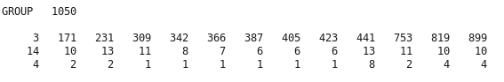 The first column gives information for the Mercury coefficients, the second for Venus and until the 9th column for Pluto. The 10th column gives information for the Moon and the 11th for the Sun. Each column contains the following information:
- the starting location of the coefficients in the data record
- the number of Chebyshev coefficients per component
- the number of complete sets of coefficients in each data record
The next step is the read the coefficient file itself. I opened the file "ascp1960.405". Each coefficient file contains multiple records. These records are split by lines which contain exactly 2 numbers, i.e. "1 1018". The first 2 numbers in each record are the start and end dates given in Julian days. The remaining entries in the data record are the coefficients.
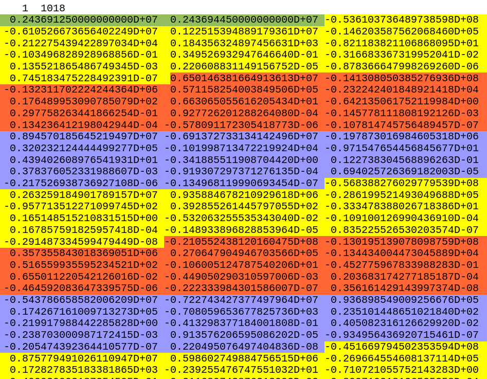 They are stored in component order, meaning that the first 14 coefficients in our case are for the $x$ component of Mercury ($a$ coefficients), the next 14 for the $y$ component ($b$ coefficients), and the next 14 for the $z$ component ($c$ coefficients). This order repeats another 3 times before starting again with Venus. For example in the above image, the yellow coefficients are the $x$ coefficients, the orange are for $y$ and the blue are for $z$.
Now we must break up the time interval. The time for the entire record goes from Julian day $2.4369125\times 10^6$ to $2.4369445\times 10^6$, but for Mercury this must be split up into 4 equal subintervals:
- $[2.4369125, 2.4369205]\times 10^6$
- $[2.4369205, 2.4369385]\times 10^6$
- $[2.4369385, 2.4369365]\times 10^6$
- $[2.4369365, 2.4369445]\times 10^6$
Code
MATLAB code to read the ephemeris file and perform some basic analysis and plots is available here.Results
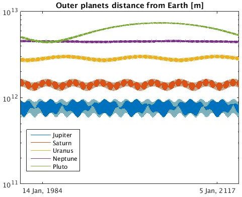
We can start by doing some basic plots of the orbits of the planets. Below is an animation of the orbits of the inner planets (period of around one Martian year): And here is one of the outer planets (period of around one Plutonian year):
 In order to compute orbital perturbations we must compute the gravitational acceleration of the celestial bodies on Earth orbiting satellites. We begin by computing the distance from each planet (and the Sun and Moon) to Earth:
\[ d = |\mathbf{x}_{\text{body}} - \mathbf{x}_{\text{Earth}}|\]
Note that in fact $\mathbf{x}_{\text{Earth}}$ is the position of the Earth-Moon barycentre. Since we know the position of the Moon, and the Earth-Moon mass ratio it is possible to compute the position of the centre of the Earth. However for practical purposes, since the distances will be so large, the difference between the actual position of the Earth and the Earth-Moon barycentre will be negligible. For the same reason, we will consider a satellite in Earth orbit to be at the Earth-Moon barycentre. This may cause some small errors in evaluating the distance from the Moon to a satellite, but will not affect an order of magnitude analysis.
In order to compute orbital perturbations we must compute the gravitational acceleration of the celestial bodies on Earth orbiting satellites. We begin by computing the distance from each planet (and the Sun and Moon) to Earth:
\[ d = |\mathbf{x}_{\text{body}} - \mathbf{x}_{\text{Earth}}|\]
Note that in fact $\mathbf{x}_{\text{Earth}}$ is the position of the Earth-Moon barycentre. Since we know the position of the Moon, and the Earth-Moon mass ratio it is possible to compute the position of the centre of the Earth. However for practical purposes, since the distances will be so large, the difference between the actual position of the Earth and the Earth-Moon barycentre will be negligible. For the same reason, we will consider a satellite in Earth orbit to be at the Earth-Moon barycentre. This may cause some small errors in evaluating the distance from the Moon to a satellite, but will not affect an order of magnitude analysis.

 Given the mass of each planet:
| Body | Mass (kg) |
| Sun | $1.989\times 10^{30}$ |
| Moon | $7.348\times 10^{22}$ |
| Mercury | $3.285\times 10^{23}$ |
| Venus | $4.867\times 10^{24}$ |
| Mars | $6.417\times 10^{23}$ |
| Jupiter | $1.898\times 10^{27}$ |
| Saturn | $5.683\times 10^{26}$ |
| Uranus | $8.681\times 10^{25}$ |
| Neptune | $1.024\times 10^{26}$ |
| Pluto | $1.309\times 10^{22}$ |

