Introduction
To a good first approximation the gravitational potential of the Earth can be approximated by: \[ U(r) = -\frac{\mu}{r}\] with:- $\mu = GM$, the gravitational parameter of the Earth ($G \approx 6.674\times 10^{-11}$ N m$^2$ kg$^{-2}$ is the gravitational constant and $M$ is the mass of the Earth)
- $r$ is the radial distance to the Earth's centre
This project is based on parts of my work at CNES, however all code and results are entirely my own.
Model
Outside of the Earth, Gauss's law for gravity tells us that the gravitational potential must satisfy the Laplace equation: \[ \Delta U = 0\] The general solution to this problem in spherical coordinates is the spherical harmonic expansion: \begin{equation}\label{eq:u} U(r, \theta, \varphi) = \frac{\mu}{r}\left(1 + \sum\limits_{n = 1}^\infty \left(\frac{a}{r}\right)^n \sum\limits_{m=0}^n Y_n^m(\sin(\theta))(C_n^m\cos(m\varphi) + S_n^m\sin(m\varphi))\right) \end{equation} where:- $a$ is a scaling factor, usually taken to be the mean equitorial radius of the Earth ($a = 6378136.3$ m for EGM 96)
- $(r, \theta, \varphi)$ are the spherical coordinates of a point:
- $r$ is the radial distance to the centre of the Earth
- $\theta$ is the elevation angle
- $\varphi$ is the azimuth angle
- $Y_n^m$ is the normalized associated Legendre polynomial of degree $n$ and order $m$. They are normalized relative to $P_n^m$, the unnormalized associated Legendre polynomial, by: \[Y_n^m(x) = \sqrt{\frac{(2 - \delta_{0m})(2n + 1)(n - m)!}{(n + m)!}}P_n^m(x)\] with \[\delta_{m0} = \begin{cases}1 &\text{ if } m = 0\\ 0 &\text{otherwise}\end{cases}\]
- $C_n^m$ and $S_n^m$ are the (normalized) empirically determined coefficients, ususally called the Stokes coefficients.
For $m = 0$ we have that $\sin(m\varphi) = 0$, so often the potential is written as: \begin{align*} U(r, \theta, \phi) = \frac{\mu}{r}\biggl(1 &+ \sum\limits_{n = 2}^\infty \left(\frac{a}{r}\right)^n J_n Y_n^0(\sin(\theta)) \\&+ \sum\limits_{n=2}^\infty\sum\limits_{m=1}^n \left(\frac{a}{r}\right)^n Y_n^m(\sin(\theta))(C_n^m\cos(m\varphi) + S_n^m\sin(m\varphi))\biggr) \end{align*} Here the $J$ coefficients are called the zonal coefficients. The zonal terms depend only on the latitude. The $J_2$ term is the largest perturbing term and represents the fact that the Earth is actually an ellipsoid with a bulging equator instead of a sphere. The $C$ and $S$ coefficients are called sectorial if $n=m$ and tesseral if $n\ne m$.
Code
MATLAB code for the EGM 96 model is available here.Results
Geoid Undulation
The geoid is defined as the equipotential surface which best fits (in a least squared sense) mean sea level. The geoid undulation is the difference between this equipotential surface and an ellipsoid which bests fits the shape of the Earth.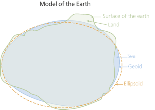 To calculate the geoid undulation we first calculate the ellipsoidal normal potential $V$:
\[ V(r,\theta,\varphi) = -\frac{\mu}{r}\left(1 + \sum\limits_{n \text{ even}}^\infty\left(\frac{a}{r}\right)^n J_n Y_n^0(\sin(\theta))\right).\]
We take the even zonal terms because these are symmetric around the equator. We then can subtract this from the potential $U$ to get the disturbing potential $T$:
\[ T(r,\theta,\varphi) = U(r,\theta,\varphi) - V(r,\theta,\varphi).\]
The geoid undulation is related to the disturbing potential by Bruns' formula:
\[ N = \frac{T}{\gamma}\]
where $\gamma$ is the magnitude of the normal gravity on the surface of the ellipsoid. In a spherical approximation, on the surface of the Earth ($r = a$) the magnitude of the normal gravity is simply $\gamma \approx \mu/a^2$. This gives the undulation:
\[ N(a, \theta,\varphi) = \frac{a^2}{\mu}T(a,\theta,\varphi).\]
Plotting $N$ over a map of the Earth:
To calculate the geoid undulation we first calculate the ellipsoidal normal potential $V$:
\[ V(r,\theta,\varphi) = -\frac{\mu}{r}\left(1 + \sum\limits_{n \text{ even}}^\infty\left(\frac{a}{r}\right)^n J_n Y_n^0(\sin(\theta))\right).\]
We take the even zonal terms because these are symmetric around the equator. We then can subtract this from the potential $U$ to get the disturbing potential $T$:
\[ T(r,\theta,\varphi) = U(r,\theta,\varphi) - V(r,\theta,\varphi).\]
The geoid undulation is related to the disturbing potential by Bruns' formula:
\[ N = \frac{T}{\gamma}\]
where $\gamma$ is the magnitude of the normal gravity on the surface of the ellipsoid. In a spherical approximation, on the surface of the Earth ($r = a$) the magnitude of the normal gravity is simply $\gamma \approx \mu/a^2$. This gives the undulation:
\[ N(a, \theta,\varphi) = \frac{a^2}{\mu}T(a,\theta,\varphi).\]
Plotting $N$ over a map of the Earth:
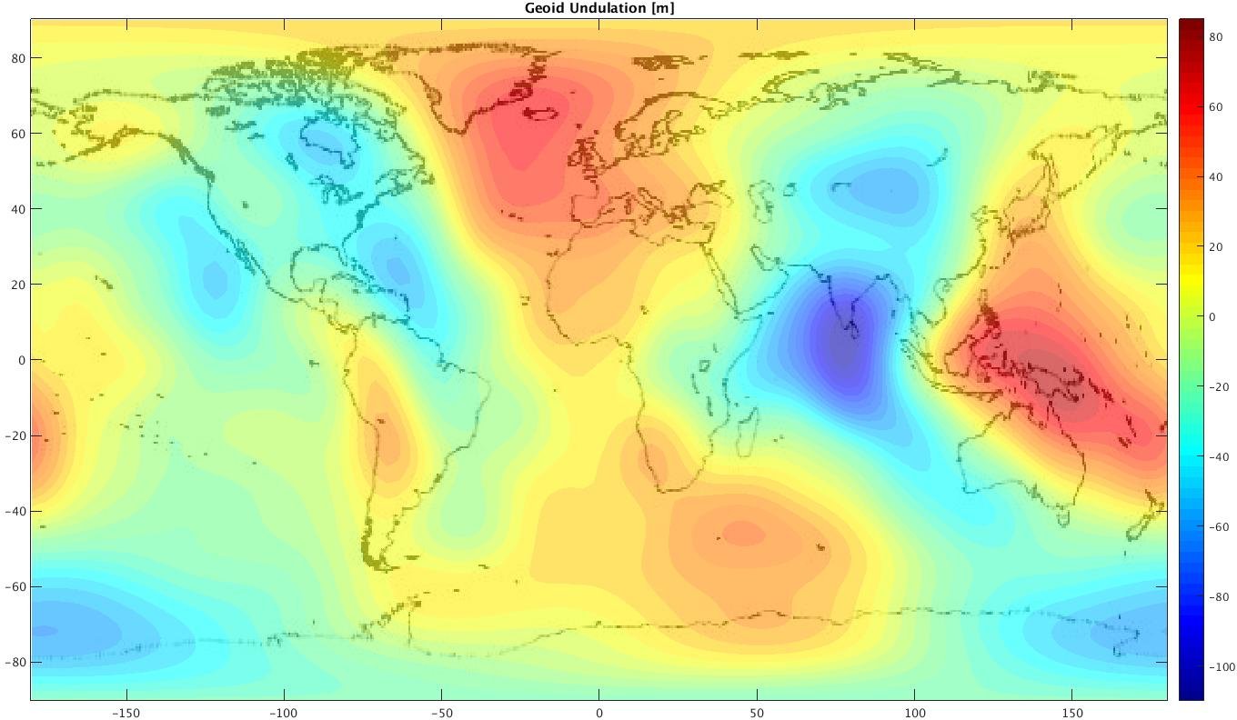 This map seems to compare well (at least visually) to those maps produced by other research. On our map, as well as in the the link provided, you can see the low area around India and the high areas around Iceland and northern Australia quite clearly. The magnitudes of the undulations seem to be consistent as well.
Gravitational Perturbations
In orbit propagation we are interested in how the potential $U(r,\theta,\varphi)$ affects the acceleration on the satellite. The total gravitational acceleration can be calculated from the gradient of the potential: \[ \mathbf{g} = -\nabla U\] In spherical coordinates the gradient is given by \[ \nabla f = \frac{\partial f}{\partial r}\mathbf{\hat{r}} + \frac{1}{r}\frac{\partial f}{\partial \theta}\mathbf{\hat{\theta}} + \frac{1}{r\sin\theta}\frac{\partial f}{\partial \varphi}\mathbf{\hat{\varphi}}\] Using the definition of U in \eqref{eq:u}, we have: \begin{align*} &g_r = -\frac{\mu}{r^2} - \sum\limits_{n=1}^\infty \frac{\mu(n+1) a^n}{r^{n+2}}\sum\limits_{m=0}^n Y_n^m(\sin(\theta))(C_n^m\cos(m\varphi) + S_n^m\sin(m\varphi))\\ &g_\theta = \sum\limits_{n = 1}^\infty \frac{\mu a^n}{r^{n+2}} \sum\limits_{m=0}^n \frac{\text{d}}{\text{d} \theta}Y_n^m(\sin(\theta))\cos(\theta)(C_n^m\cos(m\varphi) + S_n^m\sin(m\varphi))\\ &g_\varphi = \sum\limits_{n = 1}^\infty \frac{\mu a^n}{r^{n+2}\sin\theta} \sum\limits_{m=0}^n mY_n^m(\sin(\theta))(S_n^m\cos(m\varphi) - C_n^m\sin(m\varphi)) \end{align*} This formulation of the acceleration has singularities at the equator ($\theta = 0$) and at the poles ($\theta = \pm \pi / 2$). These singularities can be avoided in several ways; for example see this article by Cunningham.We are interested in the difference between this total acceleration, and that predicted by a perfectly spherical Earth: \[ g_{\text{pert}}(r,\theta,\varphi) = -\nabla U(r,\theta,\varphi) - \frac{\mu}{r^3}\mathbf{\hat{r}}.\] Overlaying $|g_{\text{pert}}|$ on a map of Earth for $r = a + 2\times 10^6$ m:
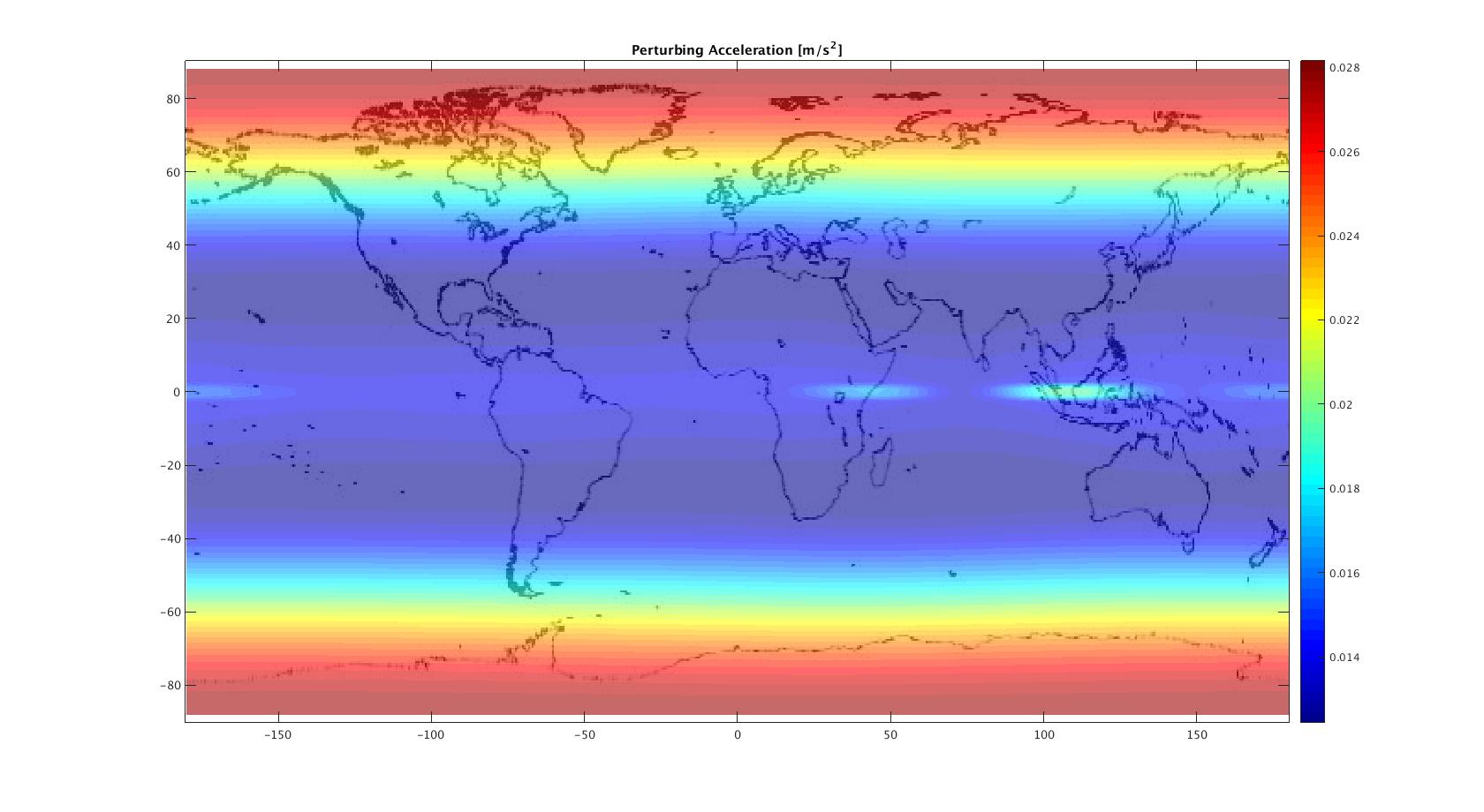 As expected the bulk of the perturbations are due to the bulging equator of the Earth.