Introduction
Error estimates are an important part of finite element analysis. For a polygonal domain $\Omega$, if our exact solution $u$ is in the space $H^{k+1}(\Omega)$, then if we use Lagrangian elements of order $k$ the following error estimates holds: \begin{align*} ||u - u^h||_0 &\leq C h^{k+1}||u||_{k+1}\\ ||u - u^h||_1 &\leq C h^k ||u||_{k+1} \end{align*} The reason this holds on polygonal domains is that we are are able to mesh the domain exactly using regular triangular or quadrilateral elements. On general curved domains we are no longer able to do this, thus our error also depends on how well our elements cover the actual domain.Curvilinear Elements
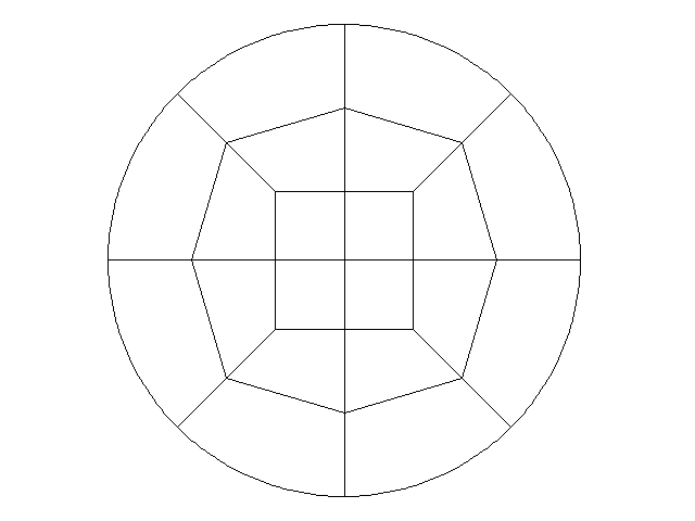
One possible way to alleviate this problem is to use higher order mappings. When we evaluate basis functions on polygonal meshes, we use a linear map to map the basis function from the reference element to the element of interest. We can use higher order mappings to map from a reference element with straight edges (square or triangle) to one with curved edges.Results
Consider the Poisson equation, \[ \Delta u = f \text{ in }\Omega,\qquad u = g \text{ on } \partial\Omega.\] We will use the method of manufactured solutions to test the convergence of various elements and mappings on a circle. Specifically we will use the radially symmetric Gaussian given by \[ u(r) = e^{-r^2},\] with $r=\sqrt{x^2+y^2}$. The boundary condition $g$ on the unit circle is then $g = u(1)$.$Q_1$ Elements
We will begin with bilinear $Q_1$ elements and a regular linear mapping.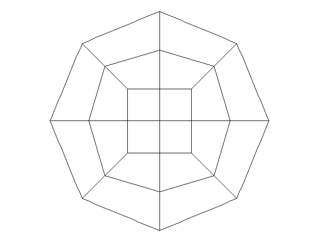
| $h$ | degrees of freedom | $||u - u^h||_0$ | rate | $||u - u^h||_1$ | rate |
| $1.082\times 10^{0}$ | 8 | $3.143\times 10^{-1}$ | - | $5.585\times 10^{-1}$ | - | $7.097\times 10^{-1}$ | 25 | $9.487\times 10^{-2}$ | 1.73 | $3.272\times 10^{-1}$ | 0.77 |
| $4.041\times 10^{-1}$ | 89 | $2.471\times 10^{-2}$ | 1.94 | $1.708\times 10^{-1}$ | 0.94 |
| $2.117\times 10^{-1}$ | 337 | $6.249\times 10^{-3}$ | 1.98 | $8.653\times 10^{-2}$ | 0.98 |
| $1.091\times 10^{-1}$ | 1313 | $1.567\times 10^{-3}$ | 2.00 | $4.342\times 10^{-2}$ | 0.99 |
With bilinear elements we are able to pick up optimal accuracy in both the $L^2$ and $H^1$ norms.
$Q_2$ Elements
We will now use $Q_2$ elements with a linear mapping.| $h$ | degrees of freedom | $||u - u^h||_0$ | rate | $||u - u^h||_1$ | rate |
| $1.082\times 10^{0}$ | 25 | $2.567\times 10^{-1}$ | - | $3.202\times 10^{-1}$ | - | $7.097\times 10^{-1}$ | 89 | $7.068\times 10^{-2}$ | 1.86 | $1.264\times 10^{-1}$ | 1.34 |
| $4.041\times 10^{-1}$ | 337 | $1.749\times 10^{-2}$ | 2.02 | $4.642\times 10^{-2}$ | 1.44 |
| $2.117\times 10^{-1}$ | 1313 | $4.297\times 10^{-3}$ | 2.02 | $1.674\times 10^{-2}$ | 1.47 |
| $1.091\times 10^{-1}$ | 5185 | $1.062\times 10^{-3}$ | 2.02 | $5.983\times 10^{-3}$ | 1.48 |
We see that the $L^2$ error is $O(h^2)$, while the $H^1$ error is $O(h^{3/2})$. This is suboptimal. We can try the same $Q_2$ elements, but with a quadratic mapping instead.
| $h$ | degrees of freedom | $||u - u^h||_0$ | rate | $||u - u^h||_1$ | rate |
| $1.082\times 10^{0}$ | 25 | $9.628\times 10^{-3}$ | - | $6.827\times 10^{-2}$ | - | $7.097\times 10^{-1}$ | 89 | $1.451\times 10^{-3}$ | 2.73 | $2.991\times 10^{-2}$ | 1.19 |
| $4.041\times 10^{-1}$ | 337 | $1.910\times 10^{-4}$ | 2.93 | $7.847\times 10^{-3}$ | 1.93 |
| $2.117\times 10^{-1}$ | 1313 | $2.421\times 10^{-5}$ | 2.98 | $1.901\times 10^{-3}$ | 2.05 |
| $1.091\times 10^{-1}$ | 5185 | $3.015\times 10^{-6}$ | 3.01 | $4.594\times 10^{-4}$ | 2.05 |
This lets us pick up the optimal accuracy. This second order element with a second order mapping is called an isoparametric element.
$Q_3$ Elements
We can also try a third order isoparametric element.| $h$ | degrees of freedom | $||u - u^h||_0$ | rate | $||u - u^h||_1$ | rate |
| $4.041\times 10^{-1}$ | 745 | $4.162\times 10^{-5}$ | - | $3.131\times 10^{-4}$ | - |
| $2.117\times 10^{-1}$ | 2929 | $3.557\times 10^{-6}$ | 3.55 | $4.866\times 10^{-5}$ | 2.69 |
| $1.091\times 10^{-1}$ | 11617 | $2.941\times 10^{-7}$ | 3.60 | $8.109\times 10^{-6}$ | 2.59 |
| $5.513\times 10^{-2}$ | 46273 | $2.454\times 10^{-8}$ | 3.58 | $1.405\times 10^{-6}$ | 2.53 |
| $2.777\times 10^{-2}$ | 184705 | $2.087\times 10^{-9}$ | 3.56 | $2.467\times 10^{-7}$ | 2.51 |
We see that the $L^2$ error is approximately $O(h^{7/2})$ while the optimal $L^2$ error for $Q_3$ elements is $O(h^4)$. In addition the $H^1$ error looks to be $O(h^{5/2})$, while the optimal $H^1$ error should be $O(h^3)$. Both these error rates are suboptimal.
This illustrates the limits of isoparametric elements, namely that for $k>2$, they do not acheive optimal accuracy.