Introduction
In order to understand the macroscopic propererties of suspensions it can be helpful to have a detailed model of the motion of the suspended particles. From this model we may be able to extract bulk properties, such as the suspension viscosity.
Problem Formulation
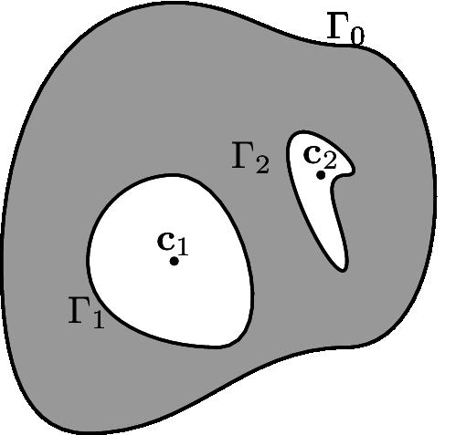
For this problem we will be considering low Reynolds number flows, which means that the governing equations will be the steady incompressible Stokes equations, given by \begin{align*} \Delta \mathbf{u} &= \nabla p,\\ \nabla\cdot\mathbf{u} &= 0. \end{align*} We will also have boundary conditions \begin{align*} \mathbf{u} &= \mathbf{u}_b \qquad\text{on } \partial\Omega,\\ \int_{\partial\Omega} \mathbf{u}_b \cdot\mathbf{n} \text{d}s &= 0 \end{align*} In a 2D simply connected domain $\Omega$ with boundary $\partial\Omega$ the solution to Stokes equations can be represented by the double layer potential \[ \mathbf{u}(\mathbf{x}) = \mathcal{D}[\pmb{\eta}](\mathbf{x}) = \frac{1}{\pi}\int_{\partial\Omega} \frac{\mathbf{r}\cdot\mathbf{n}}{\rho^2}\frac{\mathbf{r}\otimes\mathbf{r}}{\rho^2}\pmb{\eta}(\mathbf{y})\text{d}s(\mathbf{y}),\] where $\mathbf{r} = \mathbf{x}-\mathbf{y}$, $\rho = |\mathbf{r}|$ and $\pmb{\eta} = \langle \eta_1,\eta_2\rangle$ is an unknown density function.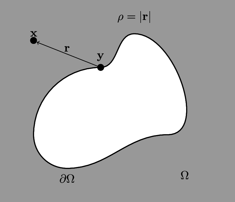 For multiply connected domain, this representation cannot pick up all possible flow fields. In general we have to add in a combination of rotlets and Stokeslets for each obstacle in the domain. The strength of the rotlet $\xi$ is the net force on the obstacle and the strength of the Stokeslet $\pmb{\lambda}$ is the net force on the obstacle.
 The rotlet represents the flow arising from a point torque at $\mathbf{y}$ and is given by \[ R(\mathbf{x},\mathbf{y})\xi = \xi\frac{\mathbf{r}^\perp}{\rho^2}.\] The Stokeslet is represents the flow arising from a point force at $\mathbf{y}$ and is given by \[ S(\mathbf{x},\mathbf{c})\pmb{\lambda} = \left(\frac{\mathbf{r}\otimes\mathbf{r}}{\rho^2} - \ln \rho\mathbf{I}\right)\pmb{\lambda}.\] Assuming $N$ obstacles, the completed double layer potential takes the form \[ \mathbf{u}(\mathbf{x}) = \mathcal{D}[\pmb{\eta}] + \sum\limits_{k=1}^N R(\mathbf{x},\mathbf{c}_k)\xi_k + S(\mathbf{x},\mathbf{c}_k)\pmb{\lambda},\] where $\mathbf{c}_k$ is a point inside obstacle $k$ (we'll take it to be the center).
We can generate a boundary integral equation by taking the limit of $\mathbf{x}$ to $\mathbf{x}^*\in\partial\Omega$ and matching this to the boundary condition $\mathbf{u}_b$. Potential theory tells us that we have a jump of -1/2 in the double layer kernel when $\mathbf{x}$ hits the boundary. This gives \[ \mathbf{u}_b(\mathbf{x}^*) = -\frac{1}{2}\pmb{\eta}(\mathbf{x}^*) + \mathcal{D}[\pmb{\eta}](\mathbf{x}^*) + \sum\limits_{k=1}^N R(\mathbf{x}^*,\mathbf{c}_k)\xi_k + S(\mathbf{x}^*,\mathbf{c}_k)\pmb{\lambda}.\]
 To close this system, we must relate the density function to the strengths of the rotlets and Stokeslets. We choose to use the relationships
\begin{align*}
\pmb{\lambda}_k &= \frac{1}{2\pi}\int_{\Gamma_k} \pmb{\eta}(\mathbf{y})\text{d}s\\
\xi_k &= \frac{1}{2\pi}\int_{\Gamma_k} (\mathbf{y}-\mathbf{c}_k)^{\perp}\cdot\pmb{\eta}(\mathbf{y})\text{d}s
\end{align*}
If we prescribe $\mathbf{u}_b$ then this is enough to solve for the density function $\pmb{\eta}$ as well as the net force and net torque on each obstacle ($\pmb{\lambda}_k$ and $\xi_k$). This is called the resistance problem. An alternative problem however is to prescribe the net force and net torque on each curve and then can solve for the $\mathbf{u}_b$. This is called the mobility problem.
To close this system, we must relate the density function to the strengths of the rotlets and Stokeslets. We choose to use the relationships
\begin{align*}
\pmb{\lambda}_k &= \frac{1}{2\pi}\int_{\Gamma_k} \pmb{\eta}(\mathbf{y})\text{d}s\\
\xi_k &= \frac{1}{2\pi}\int_{\Gamma_k} (\mathbf{y}-\mathbf{c}_k)^{\perp}\cdot\pmb{\eta}(\mathbf{y})\text{d}s
\end{align*}
If we prescribe $\mathbf{u}_b$ then this is enough to solve for the density function $\pmb{\eta}$ as well as the net force and net torque on each obstacle ($\pmb{\lambda}_k$ and $\xi_k$). This is called the resistance problem. An alternative problem however is to prescribe the net force and net torque on each curve and then can solve for the $\mathbf{u}_b$. This is called the mobility problem. For rigid bodies, we can make use no-slip boundary conditions and the fact that we can decompose the velocity at any point along the boundary into a translational ($\mathbf{u}_{\tau,k}$) and rotational component ($\omega_k$) as follows \[ \mathbf{u}_b(\mathbf{x}^*) = \mathbf{u}_{\tau,k} + \omega_k(\mathbf{x}-\mathbf{c}_k)^\perp.\] To simplify calculations we will also assume the particles are force and torque free. Once we solve for the translational and rotational velocities of each particle we can update the center and angle of each particle according to \[ \frac{\text{d}\mathbf{c}_k}{\text{d} t} = \mathbf{u}_{\tau,k} \qquad\qquad \frac{\text{d}\theta}{\text{d}t} = \omega_k.\]
Results
Unbounded Domains
If we deal properly with nearly touching particles using a near singular integration technique, we can simulate rigid fibers in an unbounded shear flow.
Bounded Domains
 Owing to the compatability condtion on boundary condition, the above formulation results in a rank one null space for bounded domains. We can remove this null space by adding the operator
\[ \mathcal{N}[\pmb{\eta}](\mathbf{x}) = \int_{\Gamma_0}(\mathbf{n}\otimes\mathbf{n})\pmb{\eta}\text{d}s.\]
This allows us to solve for example the motion of circles inside a Couette apparatus. The pressure (seen below) and the energy dissipation (seen at top of page) can be post-processed directly from the density function and the strengths of the rotlets and Stokeslets.
Owing to the compatability condtion on boundary condition, the above formulation results in a rank one null space for bounded domains. We can remove this null space by adding the operator
\[ \mathcal{N}[\pmb{\eta}](\mathbf{x}) = \int_{\Gamma_0}(\mathbf{n}\otimes\mathbf{n})\pmb{\eta}\text{d}s.\]
This allows us to solve for example the motion of circles inside a Couette apparatus. The pressure (seen below) and the energy dissipation (seen at top of page) can be post-processed directly from the density function and the strengths of the rotlets and Stokeslets.