Home

Projects

Courses

CV

DTM 94

Introduction

The Drag Temperature Model (DTM 94) described by Berger, Biancale, Ill and Barlier is an update to DTM 77. The coefficients have been updated and the model tweaked slightly to include Hydrogen, as well as higher order dependencies on the solar and geomagnetic indices.

This project is based on parts of my work at CNES, however all code and results are entirely my own.

Modifications to DTM 77

As in the DTM 77 model, temperature is defined as: \[ T(z) = T_{\infty} - (T_{\infty} - T_{120})\exp(-\sigma\xi)\] with $\xi$ defined as before, but now $\sigma$ is called the relative vertical temperature gradient and takes the form: \[\sigma = \frac{T_{120}'}{T_{\infty} - T_{120}}\] with $T_{120}'$ the known vertical temperature gradient at 120 km. As in DTM 77, $\sigma$ is constant, and we can integrate the diffusion equilibrium equation to obtain: \[ \eta_i(z) = A_{1i} \exp(G_i(L) - 1)f_i(z)\] where $\eta_i$ is the concentration of constituent $i$, now one of Hydrogen, Helium, Oxygen or molecular Nitrogen. In the paper by Berger et al $f_i(z)$ is given in the form: \[ f_i(z) = \left(\frac{T_{120}}{T(z)}\right)^{1+\alpha+\gamma_i}\exp(-\sigma\gamma_i\xi)\] which is equivalnt to the definition of $f_i(z)$ used in DTM 77.

The function $G(L)$ is the same as in DTM 77, with the following additions:

• an extra latitude term: $a_{37}P_1^0(\sin(\varphi))$
• a higher order solar activity term: $a_{38}(\bar{f} -150)^2$
• a higher order geomagnetic activity term, either:
  • $a_{39}k_p^2$ for the constituents, or
  • $a_{39}\exp(k_p)$ for the thermopause temperature$

There are 3 extra coefficients for each $G_i(L)$ bringing the total to 39. There are now 5 $G_i(L)$s to compute. The coefficients are available here in column order $T_{\infty}$, H, He, O and N$_2$.

Code

MATLAB code for the DTM 94 model is available here.

Model Data

To complete the model the following empirical constants are given in the paper:

Constant	Value	Units
$T_{120}$	380	K
$T_{120}'$	14.348	K km$^{-1}$
$\alpha$	-0.38 for H and He 0 for N$_2$ and O	-
$\beta$	1 + F1 for $T_\infty$, O, N$_2$ 1 for H and He	-

In addition the following constants are needed, though not given in the paper:

Constant	Value	Units
$g_{120}$	$9.5021268\times 10^{-3}$	km s$^{-2}$
$k$	$1.38064852\times 10^{-29}$	km$^2$ kg s$^{-2}$ K$^{-1}$
mass of H	$1.6737236\times 10^{-27}$	kg
mass of He	$6.6464764\times 10^{-27}$	kg
mass of O	$2.6567626\times 10^{-26}$	kg
mass of N$_2$	$4.651734\times 10^{-26}$	kg

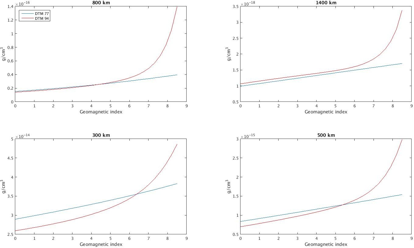
Results

Following the plots in Berger et al we can look at the sensitivity of geomagnetic index. Holding the following values fixed:

• $d = 80$
• $t = 9$
• $f = \bar{f} = 150$
• $\varphi = 45^o$

we can vary the $k_p$ to get the following plots of the density, for DTM 94 and DTM 77 at various altitudes:

Figure 2 in Berger et al

The same study repeated for the concentrations (different latitudes for He):

Figure 3 in Berger et al

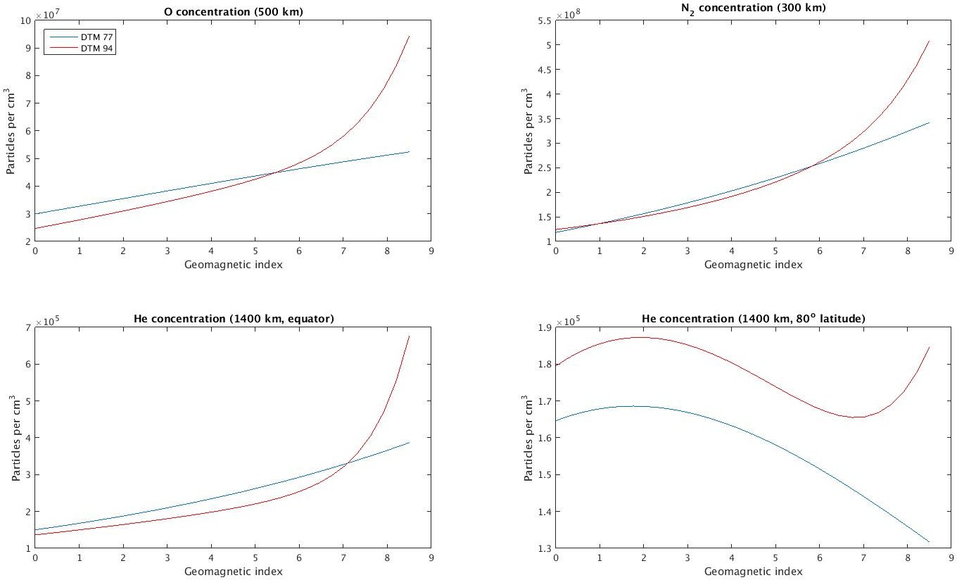And for the thermopause temperature, we can additionally look at the sensitivity to the solar flux (with $k=3$):

Figure 4 in Berger et al

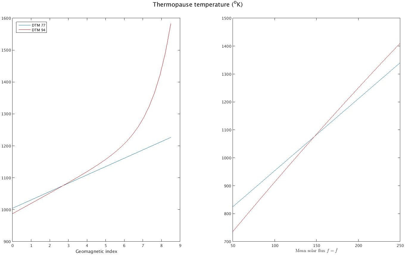Holding the other parameters fixed at the values given above, we can vary $d$:

Figure 8 in Berger et al

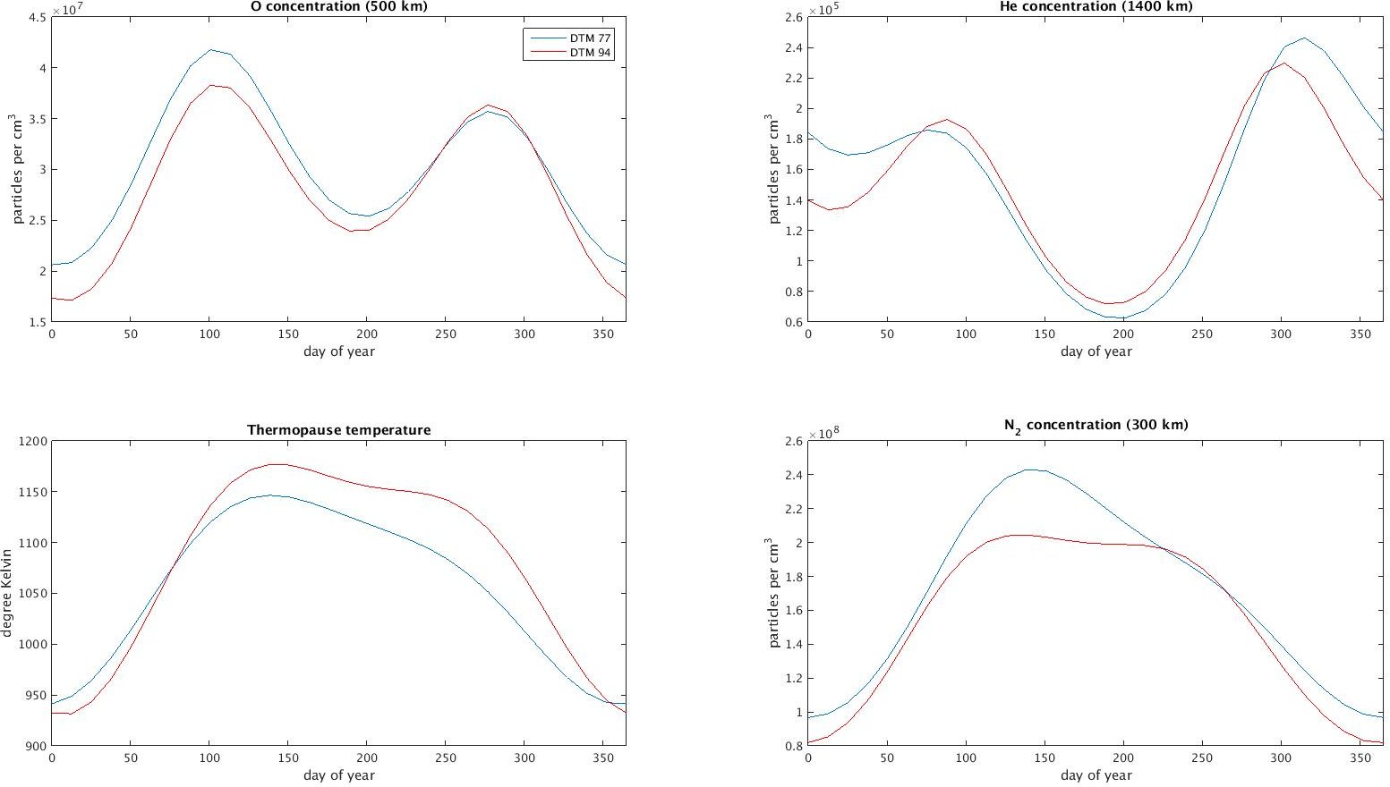And a final study, varying the latitude:

Figure 9 in Berger et al

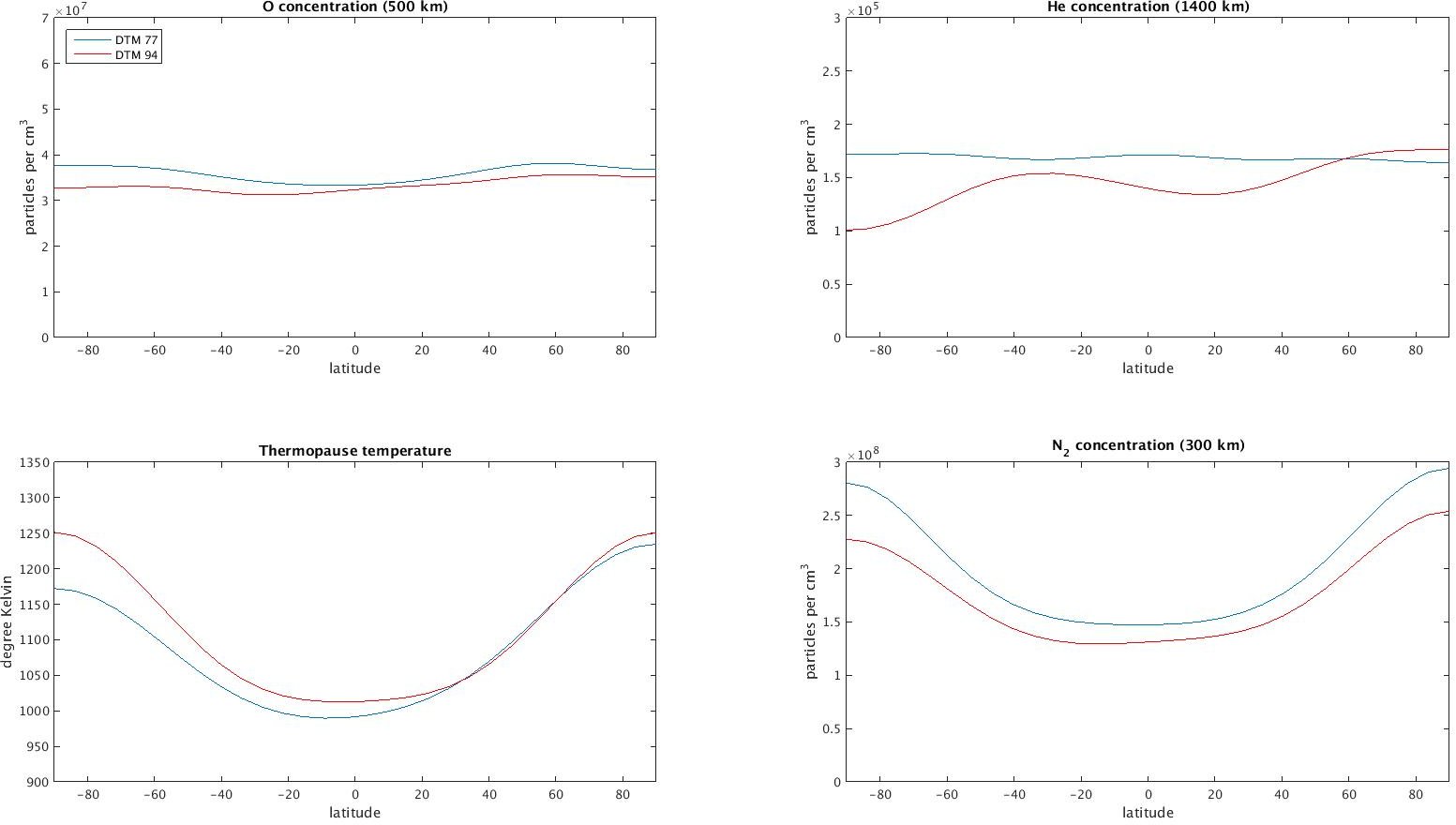A seperate paper by Bruinsma, Thuiller and Barlier provides a couple other case studies. One looks at the temperature sensitivity to solar time and latitude, while holding the following fixed:

• $d=180$
• $f = \bar{f} = 150$
• $k_p = 0$

At altitudes of $z=200$ km and $z=500$ km we can generate the following contour plots:

Figure 6 in Bruinsma et al

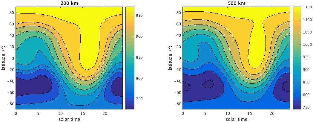We can perform a similar sensitivity study for the density, this time with the following fixed parameters:

• $d=15$
• $f = \bar{f} = 70$
• $k_p = 0$

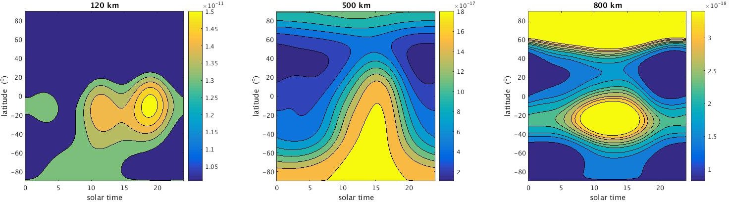Figure 9 in Bruinsma et al

Conclusions

As coded, this model replicates the results in the two papers exactly for everything except for the Helium concentration (and hence the densities, especially at the altitudes where Helium is the dominant constituent). I have not been able to reconcile this; one possibility is a typo in the provided Helium coefficients.