Introduction
The FitzHugh Nagumo (FHN) equations are an example of a nonlinear reaction diffusion system. They are given by: \begin{align} &u_t - \alpha\Delta u + u^3 - \lambda u + \sigma w + \kappa = f(\mathbf{x},t)\label{eq:fhn_1}\\ &\tau w_t - \beta\Delta w - u + w = g(\mathbf{x},t)\label{eq:fhn_2} \end{align} where $\alpha$, $\beta$, $\lambda$, $\sigma$, $\kappa$ and $\tau$ are all constants. This equation arises in cell biology and chemistry. In chemistry the functions $u(\mathbf{x},t)$ and $w(\mathbf{x},t)$ are concentrations of 2 species. In the chemistry case $u$ is an activator and $w$ is an inhibitor. We will solve this equation in 2D using finite elements.Linearization
Recall the definition of the Gâteau derivative for functions: \[ H'(X,\delta X) = \lim_{\epsilon \to 0}\frac{H(X + \epsilon\delta X) - H(X)}{\epsilon}\] Using this derivative and Newton's method we can reduce \eqref{eq:fhn_1} to the sequence of linear problems: \[ u^{k+1}_t - \alpha\Delta u^{k+1} + 3(u^k)^2u^{k+1} - \lambda u^{k+1} + \sigma w^{k+1} = f(\mathbf{x},t) -\kappa + 2 (u^k)^3\] for $k=0,1,\cdots$. Note that an initial guess for $u$, $u^0$, must be provided, but no initial guess for $w$ is necessary.Weak Formulation
First Equation
Let $U(\mathbf{x},t)$ and $W(\mathbf{x},t)$ be an approximation to $u(\mathbf{x},t)$ and $w(\mathbf{x},t)$ respectively. Multiplying by a test function $\phi_i(\mathbf{x})$ and integrating by parts: \begin{equation}\label{eq:weak} \bigl( U^{k+1}_t -\lambda U^{k+1} + 3(U^k)^2U^{k+1} + \sigma W^{k+1}, \phi_i \bigr)\ + \bigl(\alpha\nabla U^{k+1}, \nabla \phi_i\bigr) = \bigl(f(\mathbf{x},t) -\kappa + 2 (U^k)^3, \phi_i\bigr) \end{equation} Let: \[ U = \sum\limits_{i=1}^N c_j(t) \phi_j(\mathbf{x}) \qquad W = \sum\limits_{i=1}^N d_j(t) \phi_j(\mathbf{x})\] Then we can use backwards Euler to express $U_t$: \[ U_t = \sum\limits_{i=1}^N c_j'(t) \approx \frac{\sum\limits_{j=1}^N c_j^{(\ell+1)}\phi_j - \sum\limits_{j=1}^N c_j^{(\ell)}\phi_j}{\delta t}\] For $\ell = 0, \cdots, M$. Plugging $U$, $U_t$ and $W$ into \eqref{eq:weak} yields a sequence of linear problems to solve at each time step $\ell$: \begin{align*} \left(\sum\limits_{j=1}^N (1 + \delta t 3(U^k)^2 - \delta t\lambda)c_j^{(\ell+1),k+1}\phi_j , \phi_i \right) &+ \left(\delta t\sigma\sum\limits_{j=1}^N d_j^{(\ell+1),k+1}\phi_j, \phi_i\right) \\ &+ \left(\delta t \alpha\sum\limits_{j=1}^N c^{(\ell+1,)k+1}\nabla\phi_j, \nabla \phi_i\right) \\ &= \left(\delta t f(\mathbf{x}, t^{\ell+1}) -\delta t\kappa + 2\delta t (U^{(\ell+1),k})^3 + \sum\limits_{j=1}^N c_j^{(i)}\phi_j, \phi_i\right) \end{align*} Which can be written in matrix form: \[\bigl((1 - \delta t\lambda)\mathbb{M} + \delta t \alpha\mathbb{S} + \delta t\mathbb{N}^k \bigr)\mathbf{c}^{(\ell+1),k+1} + \delta t\sigma \mathbb{M} \mathbf{d}^{(\ell+1),k+1} = \left(\delta t\left(f(\mathbf{x}, t^{\ell+1}) -\kappa + 2(U^{(\ell+1),k})^3\right), \phi_i\right) + \mathbb{M}\mathbf{c}^{(\ell)}\] where:- $\mathbb{M}_{ij} = \int_\Omega \phi_j\phi_i \text{d}\Omega$
- $\mathbb{S}_{ij} = \int_\Omega \nabla\phi_j \cdot\nabla\phi_i \text{d}\Omega$
- $\mathbb{N}^k_{ij} = \int_\Omega 3(U^{(\ell+1),k})^2 \phi_j \phi_i \text{d}\Omega$
- $\mathbf{c}$ and $\mathbf{d}$ are vectors containing all the coefficients $c_j$ and $d_j$ respectively
Second Equation
Multiplying \eqref{eq:fhn_2} by a test function $\phi_i(\mathbf{x})$ and integrating by parts: \[ \bigl(\tau W_t + W - U, \phi_i\bigr) + \bigl(\beta\nabla W, \nabla \phi_i\bigr) = \bigl(g(\mathbf{x},t), \phi_i\bigr)\] Plugging in the above definitions of $w$ and $u$ and doing a backwards Euler approximation on $w_t$ yields \[ \left(\left(\tau + \delta t\right)\sum\limits_{j=1}^N d_j^{(\ell+1)}\phi_j, \phi_i\right) + \left(\delta t\beta\sum\limits_{j=1}^N d_j^{(\ell+1)}\nabla \phi_j, \nabla\phi_i\right) - \left(\delta t\sum\limits_{j=1}^N c_j^{(\ell+1)} \phi_j, \phi_i\right) = \left(\delta t g(\mathbf{x}, t^{\ell+1}) + \tau\sum\limits_{j=1}^N d_j^{(\ell)} \phi_j, \phi_i\right)\] Or in matrix form: \[ \bigl((\tau + \delta t)\mathbb{M} + \delta t \beta\mathbb{S}\bigr)\mathbf{d}^{(\ell+1)} - \delta t\mathbb{M}\mathbf{c}^{(\ell+1)} = \bigl(\delta t g(\mathbf{x}, t^{\ell+1}), \phi_i\bigr) + \tau\mathbb{M}\mathbf{d}^{(\ell)}\]Final System
To create a matrix with a nice structure, we will number the unknown coefficients: \[ \mathbf{y}^{(\ell),k} = \begin{pmatrix} c_1^{(\ell),k}, & d_1^{(\ell),k}, & c_2^{(\ell),k}, & d_2^{(\ell),k}, & \cdots, & c_N^{(\ell),k},& d_N^{(\ell),k}\end{pmatrix}^T.\] We will then solve the system: \[ \left(\begin{array}{c}\mathbb{A} \\ \hline \mathbb{B}\end{array}\right)\mathbf{y}^{(\ell + 1), k+1} = \left(\begin{array}{c}\mathbf{f}^{(\ell),k} \\ \hline \mathbf{g}^{(\ell)}\end{array}\right)\] where:- $\mathbb{A}$ is a $N\times 2N$ matrix with: \[ \mathbb{A}_{ij} = \begin{cases} (1-\delta t\lambda)\mathbb{M}_{ij} + \delta t\alpha\mathbb{S}_{ij} + \delta t \mathbb{N}^k_{ij} &\quad j \text{ odd}\\ \delta t\sigma \mathbb{M}_{ij} & \quad j \text{ even}\end{cases}\]
- $\mathbb{B}$ is a $N\times 2N$ matrix with: \[\mathbb{B}_{ij} = \begin{cases} -\delta t\mathbb{M}_{ij} &\quad j \text{ odd}\\ (\tau + \delta t)\mathbb{M}_{ij} + \delta t\beta \mathbb{S}_{ij} &\quad j \text{ even}\end{cases}\]
- $\mathbf{f}^{(\ell),k}$ is a vector of length $N$ with: \[ \mathbf{f}^{(\ell),k}_i = \left(\delta t\left(f(\mathbf{x}, t^{\ell+1}) -\kappa + 2(U^{(\ell+1),k})^3\right), \phi_i\right) + \mathbb{M}\mathbf{c}^{(\ell)}\]
- $\mathbf{g}^{(\ell)}$ is a vector of length $N$ with: \[\mathbf{g}^{(\ell)}_i = \bigl(\delta t g(\mathbf{x}, t^{\ell+1}), \phi_i\bigr) + \tau\mathbb{M}\mathbf{d}^{(\ell)}\]
Code
MATLAB code for a finite element approximation to the FHN equations is available here. This code supports Dirichlet or homogeneous Neumann boundary conditions on a rectangular domain.Results
Convergence Study
We can begin with a convergence study using the methods of manufactured solutions. If we assume exact solutions of the form: \begin{align*} &u(x,y,t) = e^{-t}\sin(\pi x)\cos(\pi y)\\ &w(x,y,t) = e^{-t}\cos(\pi x)\sin(\pi y) \end{align*} on the unit square $[0,0]\times[1,1]$, then we can generate forcing functions $f(x,y,t)$ and $g(x,y,t)$ as well as appropriate boundary conditions.If we solve this problem using quadratic basis functions $\phi(\mathbf{x})$ and backwards Euler, we would expect third order convergence space in the solution and second order in the derivatives; but only first order in time. Taking $\delta t = (\delta x)^3$ will let us isolate the spatial convergence rate.
Running from $t= 0$ to $t=0.003125$ we can generate following convergence table:
| $N_x = N_y$ | $\delta t$ | $||u - U||_2$ | rate | $||u_x - U_x||_2$ | rate | $||w - W||_2$ | rate | $||w_y - W_y||_2$ | rate |
| 5 | 1/64 | $3.70\times 10^{-3}$ | - | $9.19\times 10^{-2}$ | - | $3.70\times 10^{-3}$ | - | $9.19\times 10^{-2}$ | - |
| 9 | 1/512 | $4.63\times 10^{-4}$ | 2.99 | $2.31\times 10^{-2}$ | 1.99 | $4.63\times 10^{-4}$ | 2.99 | $2.31\times 10^{-2}$ | 1.99 |
| 17 | 1/4096 | $5.78\times 10^{-5}$ | 3.00 | $5.79\times 10^{-3}$ | 1.99 | $5.78\times 10^{-5}$ | 3.00 | $5.79\times 10^{-3}$ | 1.99 |
This agrees with our theoretical predictions for finite elements using quadratic basis functions.
Spots and Labyrinths
Now that we are confident our code works, we can use it to try and replicate the some of the results here. Using the following constants:| $\alpha$ | 0.00028 |
| $\beta$ | 0.005 |
| $\tau$ | 1 |
| $\lambda$ | 1 |
| $\sigma$ | 1 |
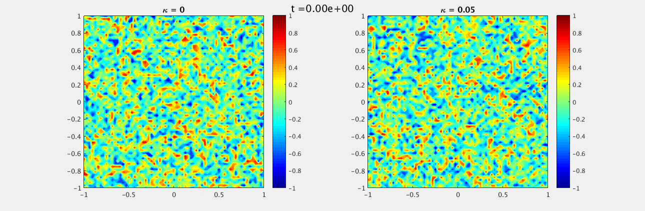
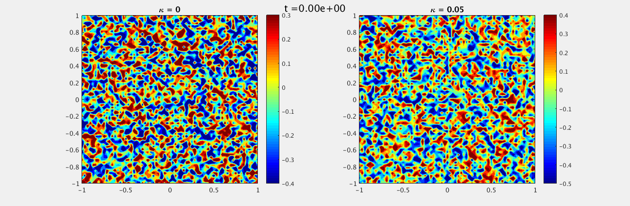
We choose a random field, uniformly distributed between -1 and 1, as our initial conditions for both $u$ and $w$. The boundary conditions on the domain $[-1,-1]\times[1,1]$ are homogeneous Neumann and we look at $t\in [0,15]$ with $\delta t = 0.1$ and $N_x = N_y = 33$. For $\kappa = 0$ we see a labyrinth pattern emerge while for $\kappa = 0.05$ there are distinct unconnected spots.
For $u$:
 For $w$:
 These look similar to the plots we expected, however there are some differences due to the random initial conditions, as well as the solver being used. In addition I was unable to find the second value of $\kappa \ne 0$ listed in the document.