Introduction
Fast Fluid Dynamics (FFD) is a technique for solving the incompressible Navier-Stokes equations. Originally developed by Jos Stam as a technique for real-time fluid visualization in video games, it has since been extended to wind load optimization among other applications. This method has the advantage of being very fast to run and relatively simple to code.The Navier-Stokes equations describe the motion of a fluid. For an incompressible fluid, the time dependent non-dimensional equations on the domain $\Omega$ with boundary $\Gamma$, over the time interval $[0,T]$, are given by: \begin{align} &\mathbf{u}_t -\nu\Delta \mathbf{u} + \mathbf{u}\cdot\nabla\mathbf{u} + \nabla p = \mathbf{f}(\mathbf{x},t)\label{eq:ns_1}\\ &\nabla\cdot\mathbf{u} = 0\label{eq:ns_2}\\ &\mathbf{u}(\mathbf{x},t) = \mathbf{g}(\mathbf{x},t) & \text{on }\Gamma \label{eq:bc}\\ &\mathbf{u}(\mathbf{x},0) = \mathbf{u}_0(\mathbf{x}) &\text{on } \Omega \label{eq:ic} \end{align} where:
- $\mathbf{u}$ is the velocity of the fluid. In 2D $\mathbf{u} = \langle u, v\rangle$
- $p$ is the fluid pressure
- $\mathbf{f}(\mathbf{x},t)$ is a known forcing function
- $\mathbf{g}(\mathbf{x},t)$ is the boundary condition
- $\mathbf{u}_0(\mathbf{x})$ is the initial condition
- $\nu$ is the kinematic viscosity of the fluid
Projection
FFD is an example of a projection method. The Hemholtz-Hodge Decomposition states that any vector field $\mathbf{w}$ can be uniquely decomposed into a vector with zero divergence and a vector with zero curl. This can be written as: \begin{equation}\label{eq:hh} \mathbf{w} = \mathbf{u} + \nabla q,\end{equation} where $\nabla\cdot\mathbf{u} = 0$ and $\nabla\times\nabla q = 0$, since all gradient fields are irrotational. Taking the divergence of both sides of \eqref{eq:hh} gives: \begin{equation}\label{eq:poisson} \nabla\cdot\mathbf{w} = \nabla\cdot\mathbf{u} + \nabla\cdot\nabla q = \Delta q.\end{equation} This is simply the Poisson equation for the scalar $q$, with the boundary condition $\nabla q\cdot\mathbf{n} = 0$, i.e. homogeneous Neumann boundary conditions. Once we have $q$, we can get $\mathbf{u}$ from \eqref{eq:hh}: \begin{equation}\label{eq:hh_u} \mathbf{u} = \mathbf{w} - \nabla q.\end{equation}Define $\mathbb{P}$ to be an operator that projects a vector onto its div-free part. Then apply this operator to \eqref{eq:ns_1}: \[ \mathbb{P} \left(\mathbf{u}_t -\nu\Delta \mathbf{u} + \mathbf{u}\cdot\nabla\mathbf{u} + \nabla p\right) = \mathbb{P} \mathbf{f}.\] Note that if $\mathbf{u}$ is smooth enough, $\nabla\cdot\mathbf{u}_t = \frac{\partial}{\partial t}\nabla\cdot\mathbf{u} = 0$. Therefore $\mathbb{P} \mathbf{u}_t = \mathbf{u}_t$. Note also that $\mathbb{P}\nabla p = 0$, since $\nabla p$ is irrotational. This leads to a single equation for the velocity: \begin{equation}\label{eq:proj} \mathbf{u}_t = \mathbb{P}\left( \nu\Delta\mathbf{u} - \mathbf{u}\cdot\nabla\mathbf{u} + \mathbf{f}\right).\end{equation} Pressure does not appear in this equation, however it can be recovered after solving for the velocity.
Method
Given the initial condition \eqref{eq:ic}, we can solve \eqref{eq:proj} by marching forward in time with time step $\delta$. Assuming we know $\mathbf{u}(\mathbf{x},t)$, we can calculate $\mathbf{u}(\mathbf{x},t+\delta)$ in four steps:- resolve forcing function: $\mathbf{w}_1 = \mathbf{u}(\mathbf{x},t) + \delta \mathbf{f}(\mathbf{x},t)$
- resolve diffusion term: $\frac{\partial }{\partial t}\mathbf{w}_1 = \nu\Delta \mathbf{w}_1$. This is solved for a single time step, yielding $\mathbf{w}_1(\mathbf{x},t+\delta) = \mathbf{w}_2$.
- resolve advection term: $\mathbf{w}_3 = \mathbf{w}_2(p(\mathbf{x}, t-\delta))$, where $p$ is the path of a a fluid element. This is called a semi-Lagrangian scheme, and is based off the method of characteristics.
- project to div-free vector: $\mathbf{u}(x,t+\delta) = \mathbb{P}\mathbf{w}_3$. From \eqref{eq:poisson} $\nabla\cdot\mathbf{w}_3 = \Delta q$, which can be solved for $q$. We then find $\mathbf{u}$ from \eqref{eq:hh_u}.
Implementation
We will use finite differences to solve the PDEs and evaluate the derivatives in this method.Resolving the diffusion term requires us the solve the PDE: \[ \frac{\partial}{\partial t}\mathbf{w}_1 = \Delta \mathbf{w}_1. \] We can discretize the time derivative using the unconditionally stable backwards Euler to get: \[ \frac{\mathbf{w}_1(t+\delta) - \mathbf{w}_1(t)}{\delta} \approx \Delta\mathbf{w}_1(t+\delta) \Rightarrow (1 - \delta \Delta)\mathbf{w}_2 = \mathbf{w}_1.\] Note that at this point $\mathbf{w}_2$ must satisfy the boundary condition \eqref{eq:bc} on $\mathbf{u}$. The Laplacian operator can be discretized using second order finite differences. Solving this system will require a solving a sparse, banded linear system.
The advection term requires us to backtrace each point, based on the intermediate velocity $\mathbf{w}_2$ and then get the new velocity $\mathbf{w}_3$ to be the velocity at the backtraced point. In 2D, at each point $\mathbf{x} = (x,y)$, there is a fluid element with velocity $(u,v) = \mathbf{w}_2$. If we use a first order linear backtrace we can say that that at $t-delta$, that fluid element was at $\hat{\mathbf{x}} = (x - \delta u, y-\delta v)$. Since $\hat{\mathbf{x}}$ will in general not be on one of our finite difference nodes, we can find the velocity at $\hat{\mathbf{x}}$ by doing a bilinear interpolation of the 4 points surrounding $\hat{\mathbf{x}}$. Once we have this velocity, we set $\mathbf{w}_3(\mathbf{x},t+\delta) = \mathbf{w}_2(\hat{\mathbf{x}},t)$.
The projection step requires us to solve the Poisson equation: \[ \Delta q = \nabla\cdot\mathbf{w}_3,\] with homogeneous Neumann boundary conditions. We can find $\nabla\cdot\mathbf{w}_3$ using second finite differences, then discretize the Laplacian operator using second order finite differences to yield another sparse, banded linear system. This linear system will actually be singular, since $q$ the boundary conditions imply that $q$ is only determined up to a constant. This can be resolved by fixing $q$ at a single point. Once we have $q$ we can find its gradient, again using second order finite differences, and subtract this from $\mathbf{w}_3$ to get $\mathbf{u}(t +\delta)$.
Lid Driven Cavity
The lid driven cavity problem is a popular test for CFD code because it is simple to implement as it requires a square domain, simple boundary conditions and no forcing function. There is also plenty of published results to compare to.A MATLAB implementation of a FFD solve of the lid driven cavity problem is available here. There are of course plenty of improvements which can be made to this code. For example, in Stam's original paper he uses a second order Runge-Kutta backtracer to evaluate the advection term. There are also more efficient solvers that can be implemented to solve the sparse linear systems.
For $Re=100$ we can look at the evolution of the $u$ component of the velocity with time:
 This simulation was done on a 32x32 grid, with $\delta = 0.01$. Once the solution reaches steady state, we can compare our results with those published by Ghia, Ghia and Shin on grids on sizes $N$x$N$:
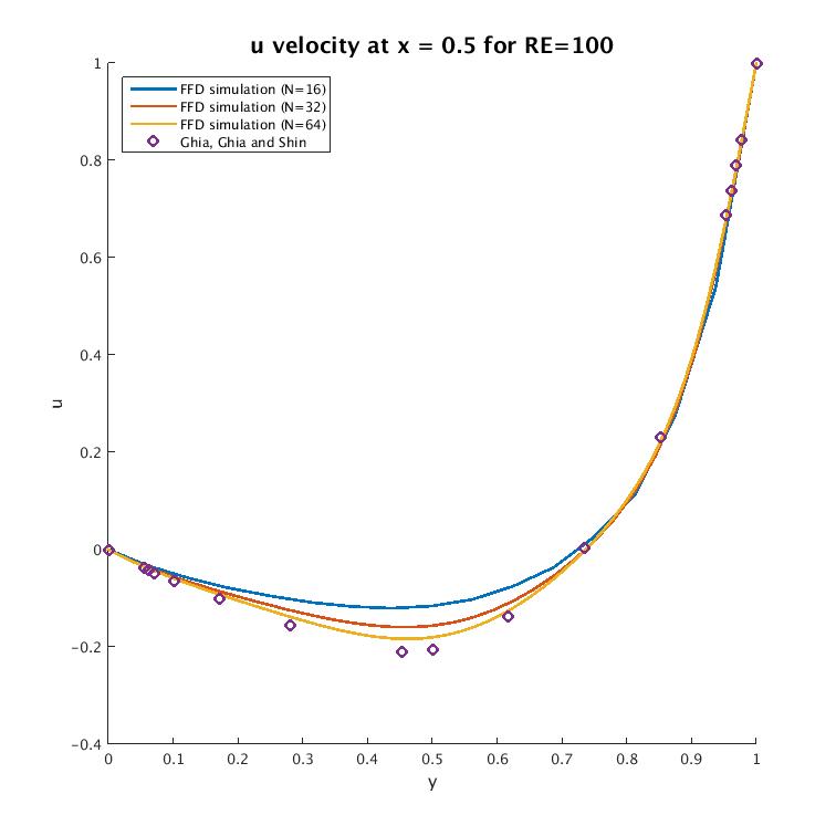 These results are fairly accurate even for a relatively coarse grid.
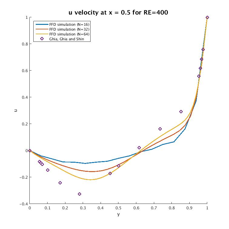
For $Re=400$ we can again look at the $u$ component over time:
 For $Re=400$ we see that the grid size plays a much larger role in the accuracy of the simulation: