Home

Projects

Courses

CV

DTM 77

Introduction

For satellites in low Earth orbit (below approximately 400 km) atmospheric drag is a large perturbing force. The atmospheric drag can be calculated from: \[ \mathbf{F}_d = -\frac{1}{2}\rho C A|\mathbf{v}|\mathbf{v}\] where:

• $\rho$ is the atmospheric density
• $C$ is the drag coefficient
• $A$ is the cross-sectional area of the satellite perpendicular to the direction of motion
• $\mathbf{v}$ is the velocity of the satellite and $|\mathbf{v}|$ is its magnitude

Accurate modelling of the atmospheric density is obviously of critical importance. Below we shall discuss the Drag Temperature Models (DTM).

This project is based on parts of my work at CNES, however all code and results are entirely my own.

Modelling Principles

For altitudes higher than 120 km, the DTM 77 model developed by Barlier, Berger, Falin, Kockarts and Thuillier in 1977 uses a spherical harmonic expansion to calculate the temperature as well as the concentrations of Helium (He), molecular Nitrogen (N$_2$) and Oxygen (O). These are all functions of altitude, latitude, solar time and solar and geomagnetic activity.

To start with we assume that we can break the atmosphere up into independent vertical columns. Inside each column the diffusive equilibrium equations holds: \begin{equation}\label{eq:equilibrium} \frac{d \eta_i}{\eta_i} = -\frac{m_i g}{k T}dz - \frac{1 + \alpha_i}{T}dT\end{equation} where:

• $\eta_i$ is the concentration of species $i$, (either He, N$_2$ or O)
• $m_i$ is the mass of species $i$
• $g$ is the acceleration due to gravity
• $k$ is the Boltzmann constant
• $T$ is the temperature
• $\alpha_i$ is the thermal diffusion factor for species $i$

Once the concentrations are calculated, the density can then be calculated from: \begin{equation}\label{eq:density}\rho = m_1\eta_1 + m_2\eta_2 + m_3\eta_3\end{equation}

Solving the Diffusive Equilibrium Equation

Let us assume a temperature profile of the following form: \[T(z) = T_\infty - (T_\infty - T_{120})\exp(-\sigma\xi)\] with:

• $T_\infty$ is the thermopause temperature
• $T_{120}$ is the constant temperature at the lower boundary of 120 km
• $\xi = \frac{(z - 120)(R + 120)}{R + z}$ is the geopoential altitude ($R$ = 6356.77 km and $z$ is measured in km)
• $\sigma = s + \frac{1}{R + 120}$, with $s$ the temperature gradient parameter

Then $\eqref{eq:equilibrium}$ can be integrated exactly to give: \begin{equation}\label{eq:concentrations} \eta_i(z) = A_{1i} \exp(G_i(L) - 1)f_i(z)\end{equation} The function $f_i(z)$ is given by: \[f_i(z) = \left(\frac{1 - a}{1 - a \exp(-\sigma\xi)}\right)^{1 + \alpha_i + \gamma_i} \exp(-\sigma\gamma_i\xi)\] with:

• $a = \frac{T_\infty - T_{120}}{T_\infty}$
• $\gamma_i = \frac{m_i g_{120}}{\sigma k T_{\infty}}$, with $g_{120}$ the gravitational acceleration at 120 km

The function $G_i(L)$ is constant in $z$. It can be expanded in terms of spherical harmonics. It will depend upon:

• the local solar time $t$
• the latitude $\varphi$
• the day count of the year $d$
• the daily 10.7 cm solar flux $f$ measured on day $d-1$
• the average solar flux $\bar{f}$ over 3 solar rotations centred on day $d$
• the three hour planetary index $k_p$ taken 3 hours before $t$.

Dropping the subscript $i$, $G(L)$ is given explicitly by: \begin{equation}\label{eq:G} \begin{aligned} G(L) = 1 + F &+ M + \sum\limits_{q = 0}^{\infty} a_q^0 P_q^0(\sin(\varphi)) \\ &+ \beta\sum\limits_{p = 1}^{\infty} b_p^0 P_p^0(\sin(\varphi))\cos(p\Omega(d - \delta_p)) \\ &+ \beta\sum\limits_{n= 1}^{\infty} \sum\limits_{m = 1}^n \left(c_n^m P_n^m(\sin(\varphi))\cos(m\omega t) + d_n^m P_n^m(\sin(\varphi))\sin(m \omega t)\right) \end{aligned} \end{equation} where:

• $\Omega = \frac{2\pi}{365 \text{ days}}$ is the approximate angular velocity of the Earth around the Sun
• $\omega = \frac{2\pi}{24 \text{ hours}}$ is the approximate rotational velocity of the Earth
• $P_i^j$ is the unnormalized associated Legendre polynomial of order $i$ and degree $j$
• The coefficients $a_q^0$, $b_p^0$, $\delta_p$, $c_n^m$ and $d_n^m$ have all been empirically calculated
• $\beta$ is a constant that depends on the constituent

The function $G(L)$ can also be used to calculate $T_{\infty}$: \begin{equation}\label{eq:temperature} T_{\infty} = A_1 G(L)\end{equation}

Reducing the Coefficients

Several simplifications will be provided below to limit the total number of coefficients to 36 for each constituent (and $T_{\infty}$). Let us rename the coefficients to $A_1, \cdots, A_{36}$. $A_1$ will be the first coefficient in \eqref{eq:concentrations} or \eqref{eq:temperature}.

The terms in $G(L)$ can be approximated as: \begin{align*} &F = A_4(f - \bar{f}) + A_5(f - \bar{f})^2 + A_6(\bar{f} - 150)\\ &M = (A_7 + A_8 P_2^0(\sin(\varphi)))k_p\\ &\sum\limits_{q = 0}^{\infty} a_q^0 P_q^0(\sin(\varphi)) \approx A_2 P_2^0(\sin(\varphi)) + A_3P_4^0(\sin(\varphi))\\ &\sum\limits_{p = 1}^{\infty} b_p^0 P_p^0(\sin(\varphi))\cos(p\Omega(d - \delta_p)) \approx AN1 + AN2 + SAN1 + SAN2\\ &\sum\limits_{n= 1}^{\infty} \sum\limits_{m = 1}^n \left(c_n^m P_n^m(\sin(\varphi))\cos(m\omega t) + d_n^m P_n^m(\sin(\varphi))\sin(m \omega t)\right) \approx D + SD + TD \end{align*} The symmetric annual term $AN1$ and the symmetric semi-annual term $SAN1$ are expressed as: \begin{align*} &AN1 = (A_9 + A_{10} P_2^0(\sin(\varphi)))\cos(\Omega(d - A_{11})\\ &SAN1 = (A_{12} + A_{13} P_2^0(\sin(\varphi)))\cos(2\Omega(d - A_{14}) \end{align*} These terms are symmetric around the equator. The annual term $AN2$ and semi-annual term $SAN2$ are anti-symmetric around the equator and are expressed as: \begin{align*} &AN2 = (A_{15}P_1^0(\sin(\varphi)) + A_{16} P_3^0(\sin(\varphi)) + A_{17}P_5^0(\sin(\varphi)))\cos(\Omega(d - A_{18})\\ &SAN2 = A_{19}P_1^0(\sin(\varphi))\cos(2\Omega(d - A_{20}) \end{align*} The diurnal term $D$ is given by: \begin{align*} D = \bigl(A_{21}P_1^1(\sin(\varphi)) &+ A_{22}P_3^1(\sin(\varphi)) + A_{23}P_5^1(\sin(\varphi)) \\ & + (A_{24}P_1^1(\sin(\varphi)) + A_{25}P_2^1(\sin(\varphi)))\cos(\Omega(d - A_{18}))\bigr)\cos(\omega t) \\ &+\bigl(A_{26}P_1^1(\sin(\varphi)) + A_{27}P_3^1(\sin(\varphi)) + A_{28}P_5^1(\sin(\varphi)) \\&+ (A_{29}P_1^1(\sin(\varphi)) + A_{30}P_2^1(\sin(\varphi)))\cos(\Omega(d - A_{18}))\bigr)\sin(\omega t) \end{align*} The semidiurnal term $SD$ is given by: \begin{align*} SD &= \left(A_{31}P_2^2(\sin(\varphi)) + A_{32}P_3^2(\sin(\varphi))\cos(\Omega(d - A_{18}))\right)\cos(2\omega t) \\ &+\left(A_{33}P_2^2(\sin(\varphi)) + A_{34}P_3^2(\sin(\varphi))\cos(\Omega(d - A_{18}))\right)\sin(2\omega t) \end{align*} Finally the tridiurnal term $TD$ is given by: \[ TD = A_{35} P_3^3(\sin(\varphi))\cos(3\omega t) + A_{36}P_3^3(\sin(\varphi))\sin(3\omega t)\]

The coefficients are available here, in column order $T_{\infty}$, He, O and N$_2$. Note that there are multiple typos in the coefficients provided in the original paper by Barlier et al.

Code

MATLAB code for the DTM 77 model is available here.

Model Data

To complete the model the following empirical constants are given in the paper:

Constant	Value	Units
$T_{120}$	380	K
$s$	0.02	km$^{-1}$
$\alpha$	-0.38 for He 0 for N$_2$ and O	-
$\beta$	1 + F1 for $T_\infty$, O, N$_2$ 1 for He	-

In addition the following constants are needed, though not given in the paper:

Constant	Value	Units
$g_{120}$	$9.5021268\times 10^{-3}$	km s$^{-2}$
$k$	$1.38064852\times 10^{-29}$	km$^2$ kg s$^{-2}$ K$^{-1}$
mass of He	$6.6464764\times 10^{-27}$	kg
mass of O	$2.6567626\times 10^{-26}$	kg
mass of N$_2$	$4.651734\times 10^{-26}$	kg

Results

We shall now test this model by recreating some of the plots in the original paper by Barlier et al.

Solar activity sensitivity

The first test we will cover the sensitivity of the temperature, density and concentrations on the solar activity. Holding fixed the following parameters:

• $d = 264$
• $\varphi = 0$
• $z = 400$ km
• $k_p = 2$

we can vary $f = \bar{f}$ and look at the daily average of the temperature, density and concentrations of He, O and N$_2$.

Figure 3 in Barlier et al

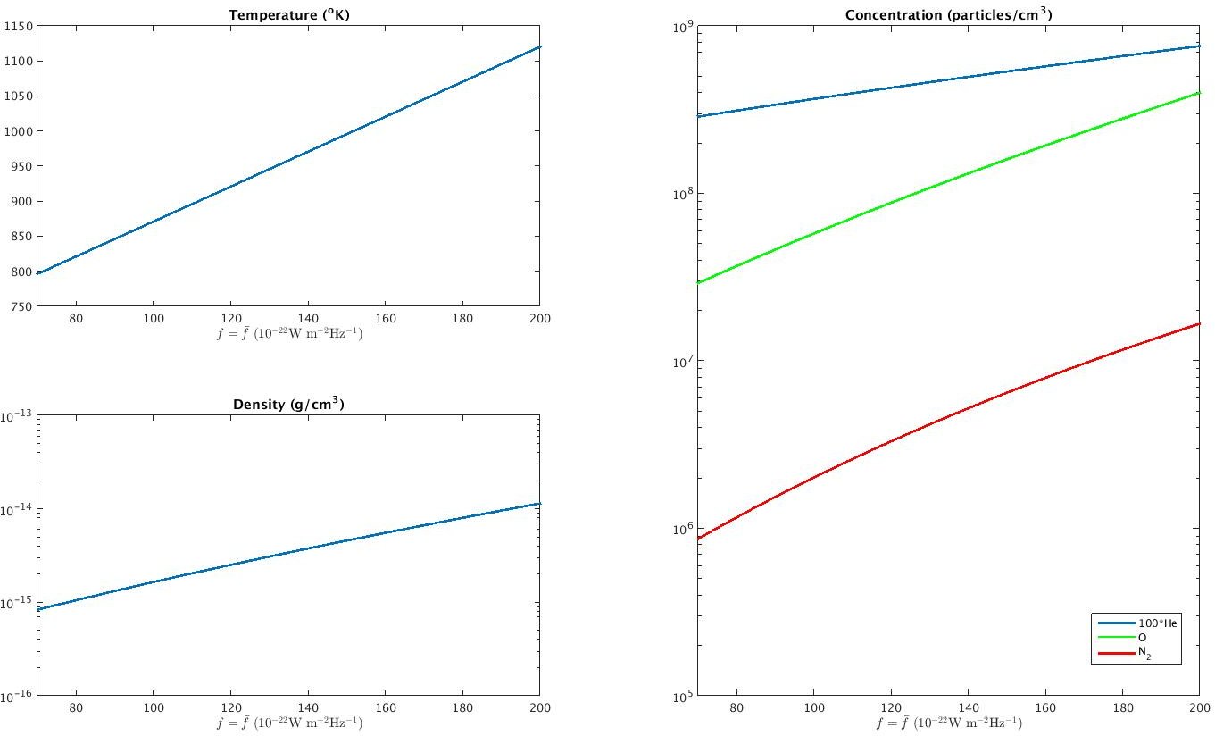Holding $\bar{f}$ constant at 130, we can vary the daily flux $f$ to study the effect of $f - \bar{f}$:

Figure 4 in Barlier et al

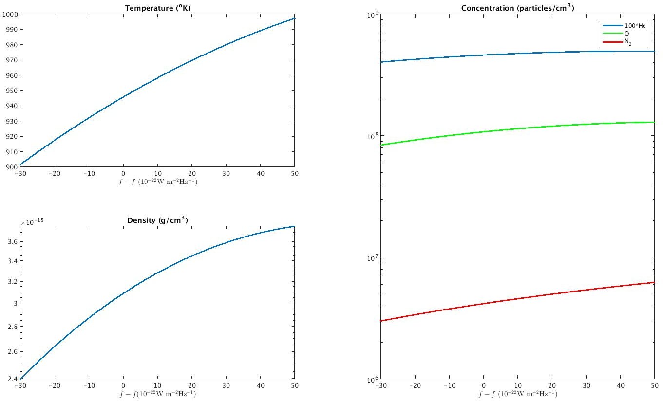Day and solar time sensitivity

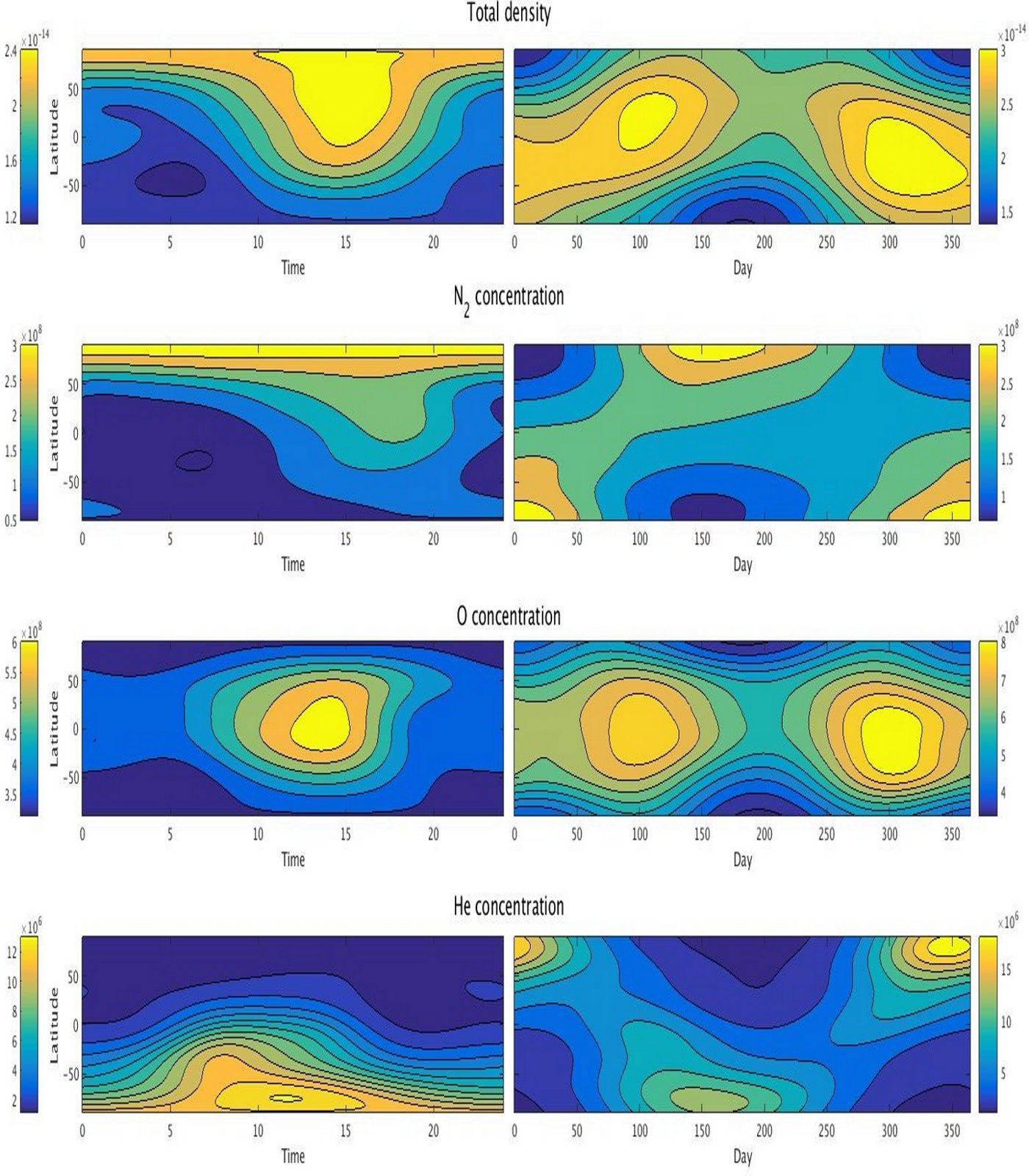
We can also look at the sensitivity of our model to the local solar time and the day of the year at various latitudes. Holding fixed the following parameters (high solar activity):

• $z = 400$ km
• $f = \bar{f} = 150$
• $k_p = 2$
• $d = 180$ when varying $t$
• $t = 15$ when varying $d$

we can generate the following contour plots:

Figure 6 in Barlier et al

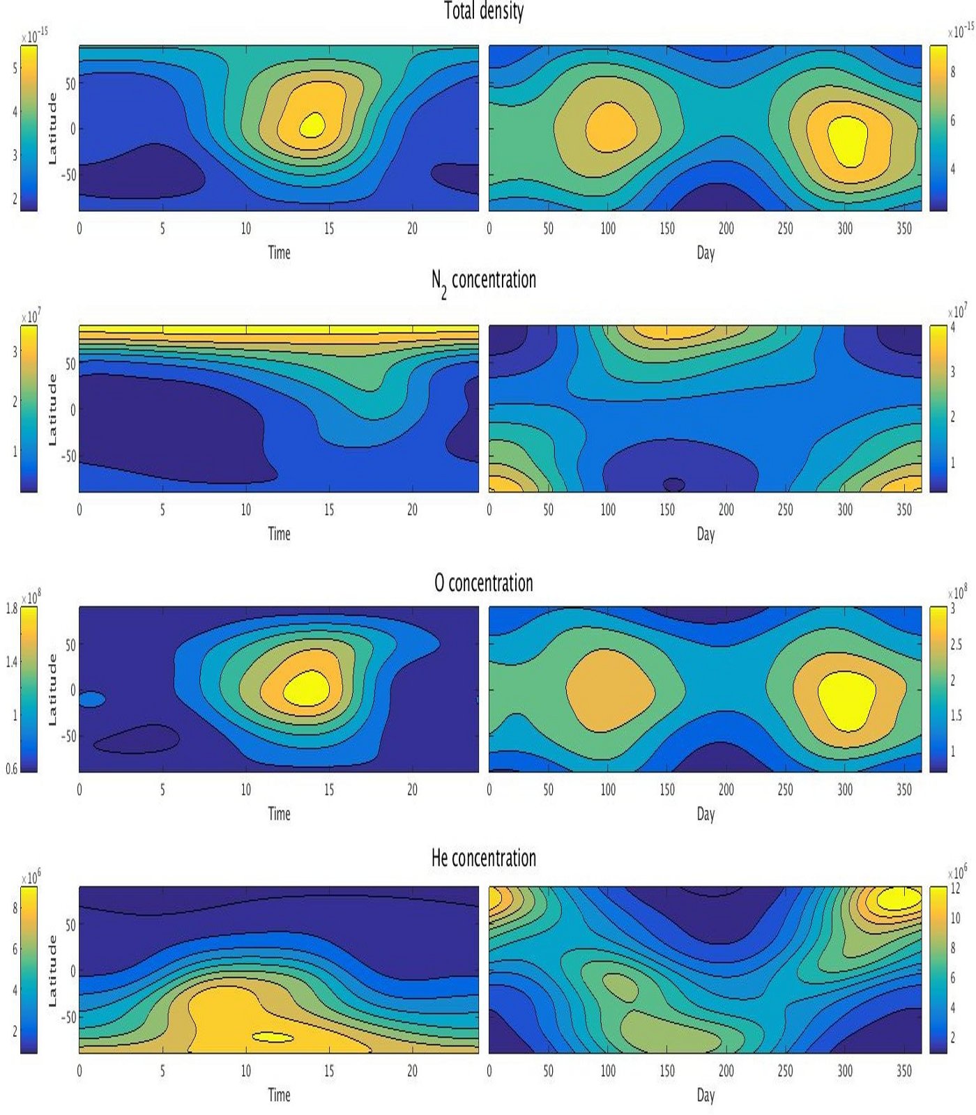For low solar activity ($f = \bar{f} = 92$, $k_p = 1$, $z = 275$ km):

Figure 7 in Barlier et al

Looking at the annual average variation at the equator for high ($f = \bar{f} = 150$, $k_p = 2$ - left) and low ($f = \bar{f} = 92$, $k_p = 1$ - right) solar activity at 400 km above the equator:

Figure 8 in Barlier et al

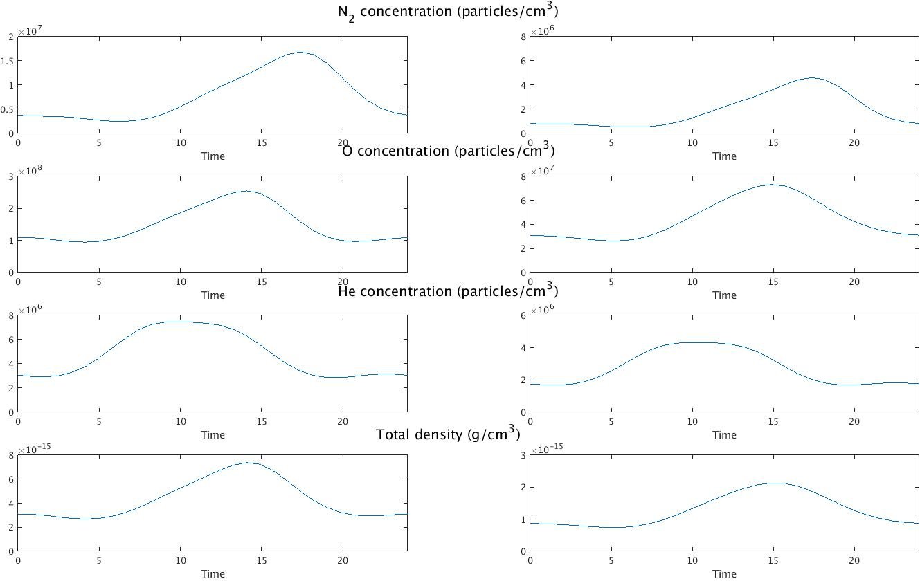Another quantity of interest is the thermopause temperature. We can see how the daily average varies over a year while holding the following conditions fixed:

• $f = \bar{f} = 150$ $10^{-22}$Wm$^{-2}$Hz$^{-1}$
• $z = 400$ km
• $k_p = 2$

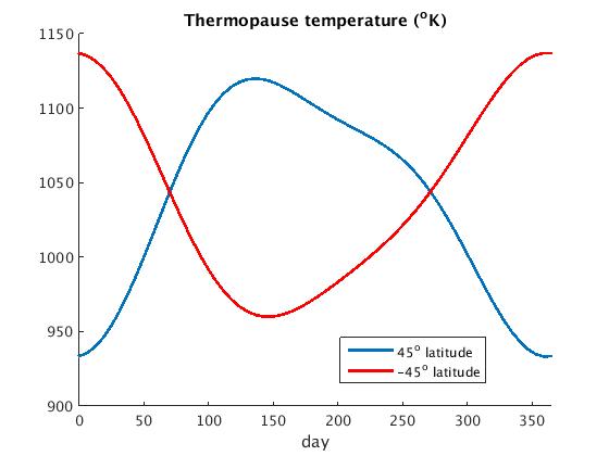Thermopause temperature variation in figure 10 in Barlier et al

Conclusions

As coded, this model replicates exactly the figures provided in Barlier et al.