gnuplot_test

gnuplot_test, a C++ code which illustrates how commands and data for the gnuplot() graphics program can be generated, to illustrate the results of a calculation.

Ordinarily, gnuplot() is used interactively; that is, the user invokes the program, and then describes the plot to be created. The data for the plot is created either by a formula, or by reference to some data file created earlier.

It is often extremely important to be able to create graphical images of the results of an executable program. If the user is familiar with gnuplot(), then the program can be modified to create a suitable data file, and, once the program has completed, the user can run gnuplot() and use that data file to create a graph.

However, if the program is going to create the data file, it can just as easily create a file containing the appropriate commands to gnuplot() that will create the desired image. In this way, the user can avoid having to recall the correct commands in the correct order to create the plot.

Thus, the program might create two files, called, perhaps data.txt and commands.txt. The command file would contain gnuplot() commands, including one that refers to the data file itself. To create the graphics image, the user would simply type

        gnuplot < commands.txt

This directory includes some sample programs which carry out numerical calculations, creating data and command files that are used in exactly this way.

Some common plot types include:

animation, a sequential display of images which are meant to suggest motion or evolution.
bar, a display of values y(1:n) in which every value y(i) is represented by a bar of that height.
bar3d, a display of values z(1:m,1:n) over a 2D grid, in which every value z(i,j) is represented by a bar of that height.
barh, a display of values x(1:n) in which every value x(i) is represented by a horizontal bar of that length. The horizontal format can be more suitable for labeling bars when there are many of them.
between, a line plot of a curve, and a filled plot of the area between the curve and the x-axis. Alternatively, a filled plot of the area between two curves.
binary_tree, a connected directed graph with no circuits, in which each node has no more than 2 descendants.
contour fill, a display of values z(x,y) in which the values of z are suggested by regions filled with color.
contour line, a display of values z(x,y) in which the values of z are suggested by colored contour lines.
decision_tree, a connected directed graph with no circuits, in which labeled nodes represent current states to be tested, and edges represent the choice or decision to move from one state to another.
dendrogram, a connected directed graph with no circuits, which generally has a single root node, and illustrates the genealogy or relatedness of a set of objects.
digraph, a "directed graph", nodes (possibly with defined locations, labels or colors), connected by directed edges (possibly with defined weights, labels, colors or linestyles).
fill, a shape composed of polygons, each of which is filled with a particular color.
graph, nodes (possibly with defined locations, labels or colors), connected by undirected edges (possibly with defined weights, labels, colors or linestyles).
heatmap, cells (typically logical squares or cubes) with an associated scalar value, such as temperature. Each cell is filled in with a color on a scale of "cold" (blue) to "hot" (red). This is related to, but different than, a colorbar or a color-filled contour map.
histogram, a display of values x in which the x range is divided into intervals, and the value y(i) represents the number of x values in the i-th interval, and a bar plot of intervals versus count is displayed.
plot, a display of a single curve defined by a sequence of functional pairs (x,y(x)), or a function y=f(x) sampled over an interval, or a sequence of related pairs (x,y).
plot3d, a 3D display of a single curve defined by a sequence of triples (x(i),y(i),z(i)), or a parametric function (x(t),y(t),z(t)) sampled over an interval.
plots, several curves on a single display.
scatter, a display of unconnected pairs (x,y), whose positions are indicated by markers.
scatter3d, a 3D display of unconnected triples (x,y,z), whose positions are indicated by markers.
scatters, a scatter plot involving several distinct sets of (x,y) pairs are displayed, distinguished by markers of different size, shape or color.
subplots, a display involving two or more separate plots, shown as a single figure.
surface, a 3D display of values z(x,y), represented as a surface.
vector, a 2D display of vectors (u,v)(x,y), representing a gradient field, an ODE direction field, or a flow of some kind.

Licensing:

The information on this web page is distributed under the MIT license.

Languages:

gnuplot_test is available in a non-language specific version and a C version and a C++ version and a Fortran77 version and a Fortran90 version and a MATLAB version and an Octave version and a Python version.

Related Data and Programs:

analemma, a C++ code which evaluates the equation of time, a formula for the difference between the uniform 24 hour day and the actual position of the sun, creating data that can be plotted by gnuplot, based on a program by Brian Tung.

brownian_motion_simulation, a C++ code which simulates Brownian motion in an M-dimensional region, creating graphics files that can be displayed with gnuplot().

disk_grid, a C++ code which computes grid points that lie inside a disk of user specified radius and center in 2D, using gnuplot() to create an image of the grid.

dislin, a C++ code which uses dislin(), a scientific graphics package, by Helmut Michels.

edge, a C++ code which defines some test functions in 1D, 2D and 3D for the detection of edges or discontinuities. It uses gnuplot() to display the jumps in curves and surfaces.

fair_dice_simulation, a C++ code which simulates N games in which two fair dice are thrown and summed, creating graphics files for processing by gnuplot.

fd1d_advection_ftcs, a C++ code which applies the finite difference method (FDM) to solve the time-dependent advection equation ut = - c * ux in one spatial dimension, with a constant velocity, using the forward time, centered space (FTCS) difference method, writing graphics files for processing by gnuplot.

fd1d_advection_lax, a C++ code which applies the finite difference method (FDM) to solve the time-dependent advection equation ut = - c * ux in one spatial dimension, with a constant velocity, using the Lax method to treat the time derivative, writing graphics files for processing by gnuplot.

fd1d_advection_lax_wendroff, a C++ code which applies the finite difference method (FDM) to solve the time-dependent advection equation ut = - c * ux in one spatial dimension, with a constant velocity, using the Lax-Wendroff method to treat the time derivative, writing graphics files for processing by gnuplot.

gnuplot_i_examples, C++ codes which demonstrate the use of the GNUPLOT_I library for interactive runtime gnuplot graphics.

high_card_simulation, a C++ code which simulates a situation in which you see the cards in a deck one by one, and must select the one you think is the highest and stop; the program uses GNUPLOT for graphics.

ising_2d_simulation, a C++ code which carries out a Monte Carlo simulation of an Ising model, a 2D array of positive and negative charges, each of which is likely to flip to be in agreement with neighbors, using gnuplot to make images of the initial and final configurations.

lebesgue, a C++ code which is given a set of nodes in 1D, and plots the Lebesgue function, and estimates the Lebesgue constant, which measures the maximum magnitude of the potential error of Lagrange polynomial interpolation, and which uses gnuplot to make plots of the Lebesgue function.

lobatto_polynomial, a C++ code which evaluates Lobatto polynomials, similar to Legendre polynomials except that they are zero at both endpoints.

lorenz_ode, a C++ code which approximates solutions to the Lorenz system, creating output files that can be displayed by Gnuplot.

naca, a C++ code which can take the parameters of certain NACA airfoils and return the coordinates of a sequence of points that outline the wing shape. The data can be displayed with gnuplot.

nearest_interp_1d, a C++ code which interpolates a set of data using a piecewise constant interpolant defined by the nearest neighbor criterion, creating graphics files for processing by gnuplot.

ornstein_uhlenbeck, a C++ code which approximates solutions of the Ornstein-Uhlenbeck stochastic ordinary differential equation (SODE) using the Euler method and the Euler-Maruyama method, and creating graphics files for processing by gnuplot.

poisson_simulation, a C++ code which simulates a Poisson process in which events randomly occur with an average waiting time of Lambda, creating output for graphics by gnuplot.

pwl_interp_1d, a C++ code which interpolates a set of data using a piecewise linear function, creating graphics files for processing by gnuplot.

sde, a C++ code which illustrates properties of stochastic ordinary differential equations (SODE), and common algorithms for their analysis, including the Euler method, the Euler-Maruyama method, and the Milstein method, making graphics files for processing and display by gnuplot, by Desmond Higham;

spiral_data, a C++ code which computes a velocity vector field that satisfies the continuity equation, writing the data to a file that can be plotted by gnuplot.

spring_ode2, a C++ code which shows how gnuplot() can illustrate a solution of the ordinary differential equation (ODE) that describes the motion of a weight attached to a spring.

stochastic_diffusion, a C++ code which implements several versions of a stochastic diffusivity coefficient, and displays sample results using gnuplot.

stochastic_heat2d, a C++ code which implements a finite difference method (FDM) for the steady (time independent) 2D heat equation, with a stochastic heat diffusivity coefficient, using gnuplot to illustrate the results.

string_simulation, a C++ code which simulates the behavior of a vibrating string, creating files that can be displayed by gnuplot.

svd_snowfall, a C++ code which reads a file containing historical snowfall data and analyzes the data with the Singular Value Decomposition (SVD), and plots created by gnuplot().

vandermonde_interp_1d, a C++ code which finds a polynomial interpolant to data y(x) of a 1D argument, by setting up and solving a linear system for the polynomial coefficients, involving the Vandermonde matrix, creating graphics files for processing by gnuplot().

Reference:

Philipp Janert,
Gnuplot in Action: Understanding Data with Graphs,
Manning, 2010,
ISBN13: 978-1-933988-39-8,
LC: QA276.4.J37.
Thomas Williams, Colin Kelley,
gnuplot 4.4, An Interactive Plotting Program,
The Free Software Foundation, 2010.
The GNUPLOT Website.

Examples and Tests:

album_bar lists the year, and total number of music albums (LP's, cassettes, CD's and downloads) sold each year from 2007 to 2017. This data is plotted as a bar graph.

album_commands.txt, the gnuplot() command file.
album_data.txt, a data file;
album_bar.cpp, reads the data and creates the gnuplot command file.
album_bar.sh, runs the test.
album_bar.txt, the output file.
album_bar.png, the plot.

automobile_scatter contains prices and weights of cars available in 1985. A scatter plot is to be made.

automobile_commands.txt, the gnuplot() command file.
automobile_data.txt, a data file.
automobile_scatter.cpp, reads the data and creates the gnuplot command file.
automobile_scatter.sh, runs the test.
automobile_scatter.txt, the output file.
automobile_scatter.png, the plot.

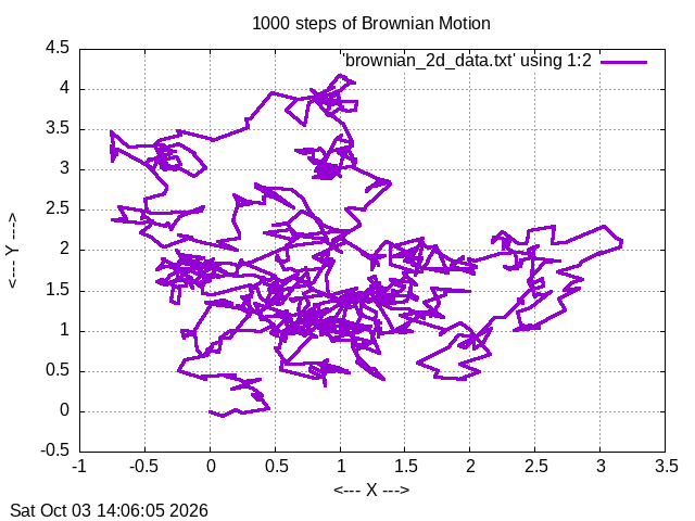
brownian_2d_plot plots data representing 1000 steps of Brownian motion in two dimensions. Unlike a typical y=f(x) plot, this data wanders around the page.

brownian_2d_commands.txt, the gnuplot() command file.
brownian_2d_data.txt, the data file.
brownian_2d_plot.cpp, plots the data
brownian_2d_plot.sh, runs the test.
brownian_2d_plot.txt, the output file.
brownian_2d_plot.png, the plot.

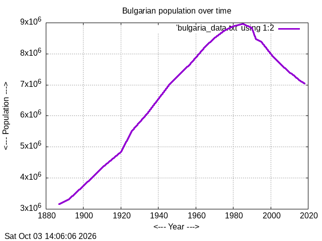
bulgaria_plot takes data about the Bulgarian population over time and makes a plot of (time,population).

bulgaria_commands.txt, the command file.
bulgaria_data.txt, a data file; each line is a year and population count.
bulgaria_plot.cpp, creates a gnuplot() command file to plot the data.
bulgaria_plot.sh, runs the test.
bulgaria_plot.txt, the output file.
bulgaria_plot.png, the plot.

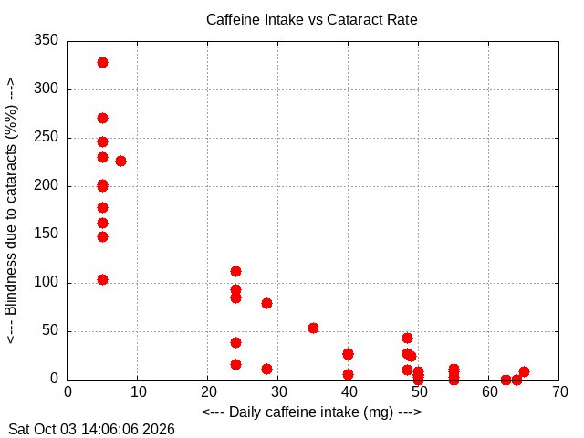
caffeine_scatter seeks a relationship between the percentage of blindness due to cataracts, and the daily intake of caffeine, in a number of countries. A scatter plot is produced.

caffeine_commands.txt, the gnuplot() command file.
caffeine_data.txt, cataract percentage, and milligrams of caffeine.
caffeine_scatter.cpp, creates a gnuplot() command file to plot the data.
caffeine_scatter.sh, runs the test.
caffeine_scatter.txt, the output file.
caffeine_scatter.png, the plot.

corkscrew_plot3d generates (X,Y,Z) points that lie along a 3D curve looking something like a corkscrew.

corkscrew_commands.txt, commands to gnuplot that will create a plot.
corkscrew_data.txt, the X, Y, Z coordinates.
corkscrew_plot3d.cpp, creates the data, and writes the GNUPLOT files.
corkscrew_plot3d.sh, runs the test.
corkscrew_plot3d.txt, the output file.
corkscrew_plot3d.png, a PNG image of the plot.

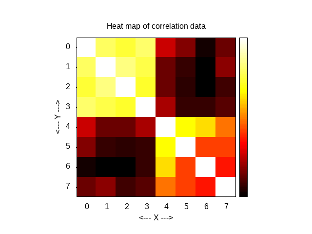
correlation_heat_map takes an 8x8 correlation matrix and draws an 8x8 grid of squares, colored white for the highest values, yellow, then red, and black for the lowest.

correlation_commands.txt, gnuplot() commands that can create an image from the data file.
correlation_heat_map.cpp, creates a heat map from a correlation matrix.
correlation_heat_map.sh, runs the test.
correlation_data.txt, the data file.
correlation_heat_map.txt, the output file.
correlation_heat_map.png, the plot.

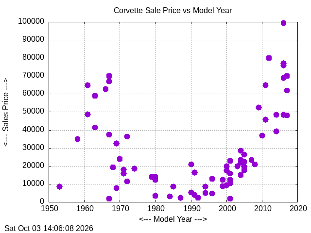
corvette_scatter considers the resale price for Corvettes by model year, displaying the results as a scatter plot.

corvette_commands.txt, commands to gnuplot that will create a plot.
corvette_data.txt, the data.
corvette_scatter.cpp, reads the data and writes the gnuplot command file.
corvette_scatter.sh, runs the test.
corvette_scatter.txt, the output file.
corvette_scatter.png, the plot.

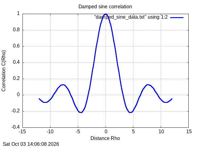
damped_sine evaluates the damped sine correlation function for a range of values of its argument. A plot of the function is desired.

damped_sine_commands.txt, gnuplot() commands that can create an image from the data file.
damped_sine_data.txt, a file containing the data values.
damped_sine_plot.cpp, the source code.
damped_sine_plot.sh, runs the test.
damped_sine_plot.txt, the output file.
damped_sine_plot.png, an image of the data.

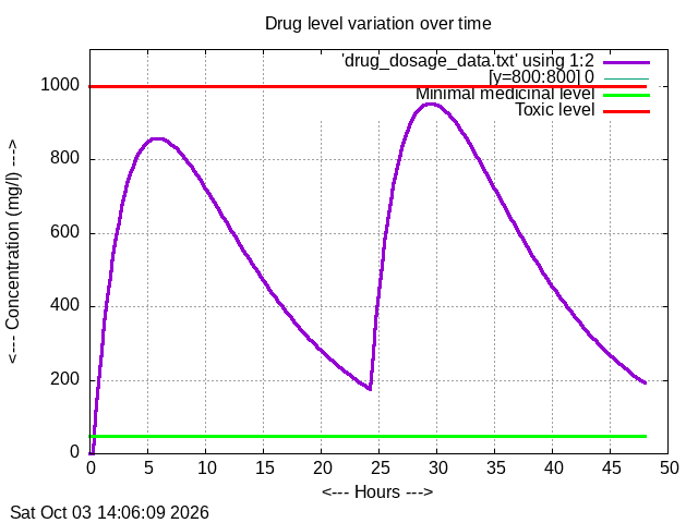
drug_dosage_plots depicts measurements over 48 hours of the blood level concentration of a medicinal drug. The drug needs to reach a certain level to have an effect, but must not exceed the toxic level. A graphic is created which shows, on one plot, the concentration over time, the minimal effective level, and the maximum nonlethal leval.

drug_dosage_commands.txt, commands to gnuplot that will create a plot.
drug_dosage_data.txt, a data file of times and concentrations;
drug_dosage_plots.cpp, reads the data, and plots the concentration level and two limiting straight lines.
drug_dosage_plots.sh, runs the test.
drug_dosage_plots.txt, the output file.
drug_dosage_plots.png, the plot.

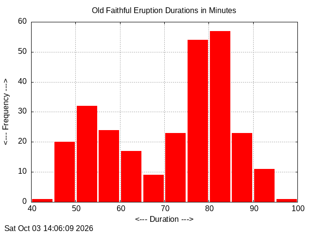
faithful_histogram contains the waiting time in minutes between successive eruptions of the Old Faithful geyser.

faithful_commands.txt, the gnuplot command file.
faithful_data.txt, waiting times and eruption durations.
faithful_histogram.cpp, reads the data and writes a gnuplot command file.
faithful_histogram.sh, runs the test.
faithful_histogram.txt, the output file.
faithful_histogram.png, the plot.

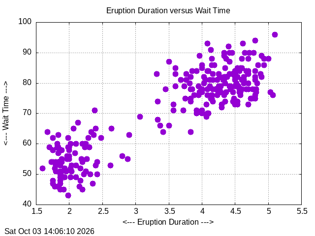
geyser_scatter looks for relations between the duration in minutes of the eruption and following waiting times for the Old Faithful geyser.

geyser_commands.txt, the gnuplot command file.
geyser_data.txt, waiting times and eruption durations.
geyser_scatter.cpp, reads the data and writes a gnuplot command file.
geyser_scatter.sh, runs the test.
geyser_scatter.txt, the output file.
geyser_scatter.png, the plot.

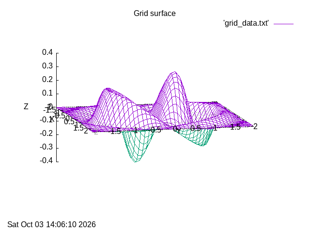
grid_surface records, on a 41x41 grid over [-2,2]x[-2,+2], the values z = exp(-(x^2+y^2)) * cos(0.25*x) * sin(y) * cos(2*(x^2+y^2)). The data is plotted as a surface.

grid_commands.txt, commands to gnuplot that will create a plot.
grid_data.txt, a table of x, y, z(x,y) values.
grid_surface.cpp, creates the data, and writes the GNUPLOT files.
grid_surface.sh, runs the test.
grid_surface.txt, the output file.
grid_surface.png, a PNG image of the plot.

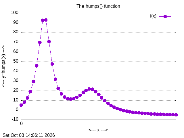
humps_plot plots the function y=humps(x) over [0,2]. Instead of a file of data, gnuplot() works directly with a formula for the function.

humps_commands.txt, the gnuplot() command file.
humps_plot.cpp, creates a gnuplot() command file to plot the data.
humps_plot.sh, runs the test.
humps_plot.txt, the output file.
humps_plot.png, the plot.

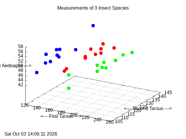
insect_scatter3d involves 3 data sets, each containing 10 measurements of 3 quantities for each of 3 species of insect. The quantities are first tarsus width, second tarsus width, and maximum width of the aedeagus. It is of interest to know whether these three measurements are enough to differentiate between members of the three species. A 3D scatter plot is created.

insect_commands.txt, commands to gnuplot that will create a plot.
insect_a_data.txt;
insect_b_data.txt;
insect_c_data.txt;
insect_scatter3d.cpp, reads the data, writes the gnuplot command file.
insect_scatter3d.sh, runs the test.
insect_scatter3d.txt, the output file.
insect_scatter3d.png, the plot.

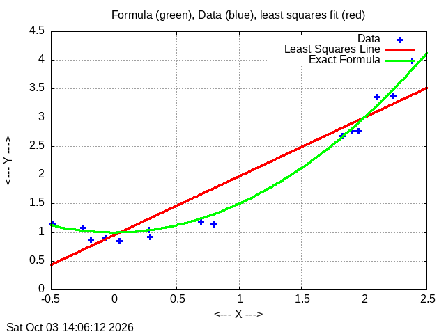
least_squares_plots compares 15 pairs of (x,y) data, the least squares line that approximates their behavior, and a quadratic curve that is much closer to the data.

least_squares_commands.txt, commands to gnuplot() that will create a plot.
least_squares1_data.txt, coordinates of the 15 sample points;
least_squares2_data.txt, coordinates of two points on the least squares approximating line;
least_squares3_data.txt, coordinates of points on the exact curve;
least_squares_plots.cpp, reads the data, writes the gnuplot command file.
least_squares_plots.sh, runs the test.
least_squares_plots.txt, the output file.
least_squares_plots.png, the plot.

mario_fill makes a simple image of Mario, by constructing a grid of squares filled with color.

mario_commands.txt, the gnuplot command file.
mario_fill.cpp, makes a command file for input to gnuplot.
mario_fill.sh, runs the test.
mario_fill.txt, the output file.
mario_fill.png, a PNG image of the plot.

mark_points adds green and red dots to mark the first and last data points in a plot.

mark_points_commands.txt, the gnuplot command file.
mark_points.cpp, makes a command file for input to gnuplot.
mark_points.sh, runs the test.
mark_points.txt, the output file.
mark_points_data.txt, the main data file.
mark_points_start_data.txt, the data file identifying the first point.
mark_points_end_data.txt, the data file identifying the last point.
mark_points.png, a PNG image of the plot.

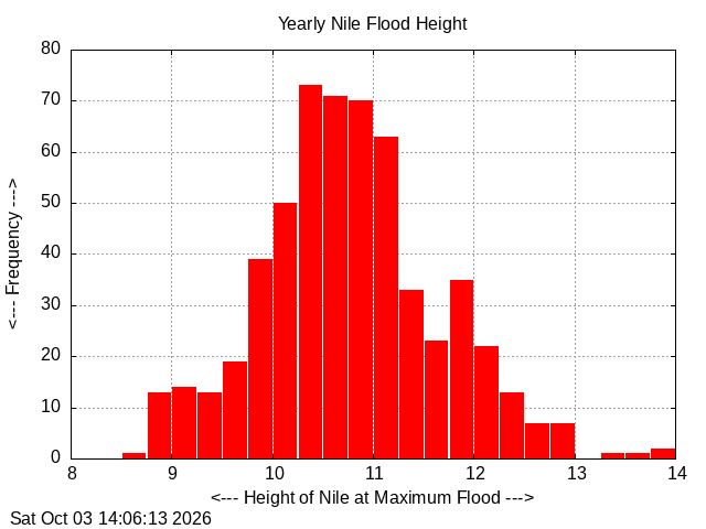
nile_histogram makes a histogram of the yearly measurement of the height of the Nile at maximum flood. By lumping the data into bins, it is easier to see the range of flood heights, and the probability of various values in the range.

nile_commands.txt, the gnuplot command file.
nile_data.txt, a list of index and flood height for each year.
nile_histogram.cpp, reads the data and writes a gnuplot command file.
nile_histogram.sh, runs the test.
nile_histogram.txt, the output file.
nile_histogram.png, the plot.

orbital_fill_contour makes a color contour plot of orbital data.

orbital_commands.txt, the gnuplot() command file.
orbital_data.txt, the gnuplot data file, formatted with blank lines between rows, to follow the gnuplot table data convention.
orbital_fill_contour.cpp, makes a command file for input to gnuplot().
orbital_fill_contour.sh, runs the test.
orbital_fill_contour.txt, the output file.
orbital_fill_contour.png, a PNG image of the plot.

predator_plot3d models the populations of predators (foxes) and prey (rabbits) over time. A 3D plot of (time, rabbits, foxes) is created.

predator_commands.txt, commands to gnuplot that will create a plot.
predator_data.txt, a list of time, prey, and predator.
predator_plot3d.cpp, creates the data, and writes the GNUPLOT files.
predator_plot3d.sh, runs the test.
predator_plot3d.txt, the output file.
predator_plot3d.png, a PNG image of the plot.

president_heights_bar plots the heights of US presidents in inches, as a bar plot.

president_heights_commands.txt, the gnuplot() command file.
president_heights_data.txt, a data file;
president_heights_bar.cpp, creates a gnuplot() command file to plot the data.
president_heights_bar.sh, runs the test.
president_heights_bar.txt, the output file.
president_heights_bar.png, the plot.

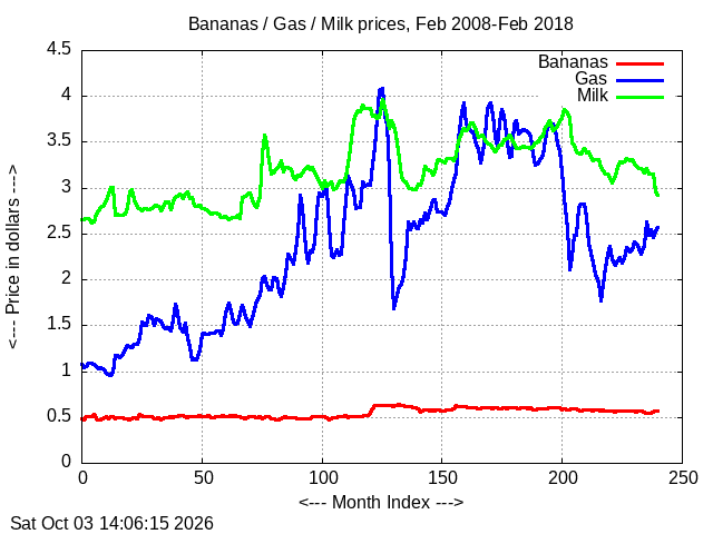
price_plots reads a table of average monthly prices for 11 consumer products, between February 2008 and February 2018, as compiled by the Bureau of Labor Statistics, and plots together the prices of three of the items.

price_commands.txt, the gnuplot() command file.
price_data.txt, a data file;
price_plots.cpp, creates a gnuplot() command file to plot the data.
price_plots.sh, runs the test.
price_plots.txt, the output file.
price_plots.png, the plot.

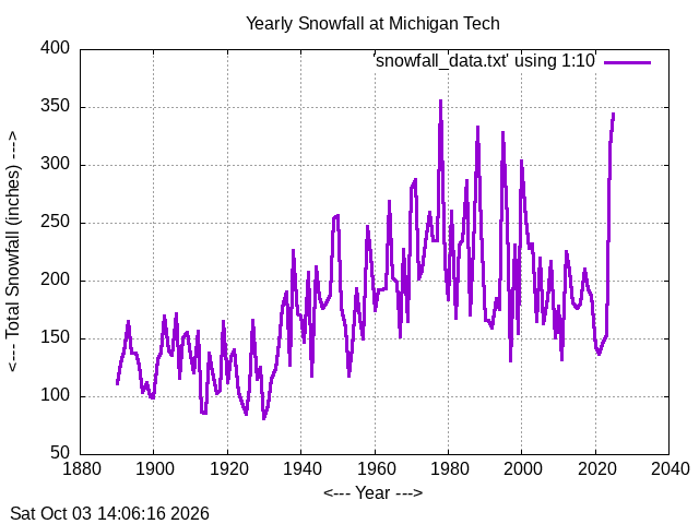
snowfall_plot makes a line plot of the snowfall at Michigan Tech from 1890 to 2017.

snowfall_commands.txt, the gnuplot() command file.
snowfall_data.txt, the data.
snowfall_plot.cpp, creates a gnuplot() command file to plot the data.
snowfall_plot.sh, runs the test.
snowfall_plot.txt, the output file.
snowfall_plot.png, the plot.

string_simulation simulates the behavior of a string that obeys the wave equation. The shape of the string is to be plotted over successive times.

string_commands.txt, gnuplot() commands that can create an image from the data file.
string_simulation.cpp, the source code.
string_simulation.txt, the output file.
string_data.txt, a file containing the data values.
string.png, an image of the data.

temperature_scatter3d shows temperatures and locations in the US where the January temperature was recorded.

temperature_data.txt, the data file, containing temperature, -longitude and latitude.
temperature_commands.txt, the gnuplot() command file.
temperature_scatter3d.cpp, creates a gnuplot() command file to plot the data.
temperature_scatter3d.sh, runs the test.
temperature_scatter3d.txt, the output file.
temperature_scatter3d.png, the plot.

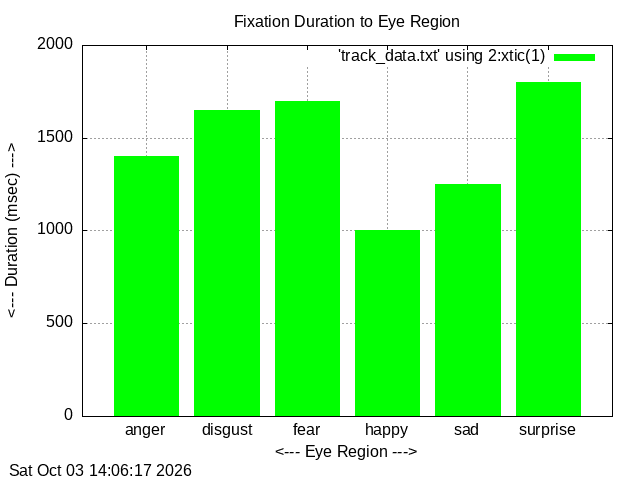
track_bar considers an eye-tracking experiment in which the eye was focused on different regions for different durations. Each region has a text label. A bar graph is desired, in which the bar for each duration is given the appropriate label.

track_commands.txt, the gnuplot() command file.
track_data.txt, a data file including a region name, and a duration;
track_bar.cpp, creates a gnuplot() command file to plot the data.
track_bar.sh, runs the test.
track_bar.txt, the output file.
track_bar.png, the plot.

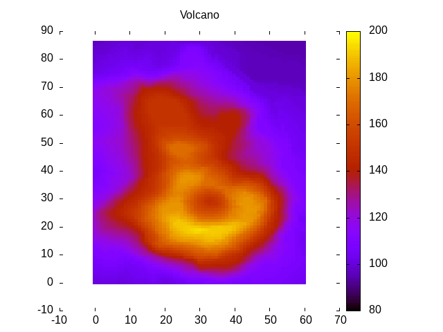
volcano_fill creates a color-filled contour plot of a volcano's height, using an MxN table of data.

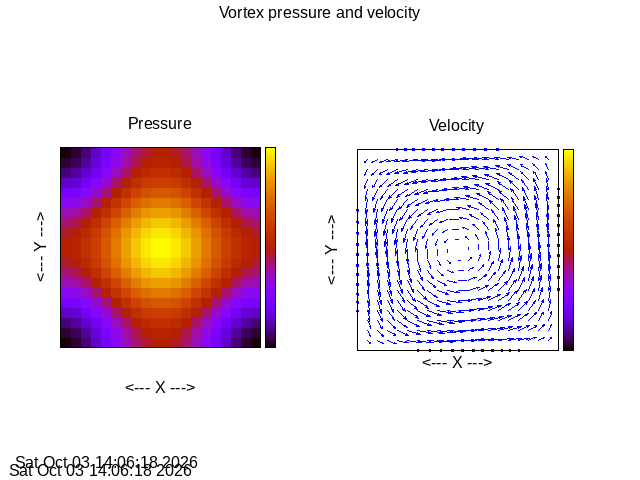
vortex_subplots shows pressure and velocity vector subplots in a single figure.

Last revised on 29 September 2026.