bvp4c_test, a MATLAB code which calls bvp4c(), which solves boundary value problems (BVP) in one spatial dimension.
A simple two point boundary value problem involves a second degree differential equation
y"(x) = f(x,y)
which is to hold over some interval
a < x < b
with
boundary conditions
        y(a) = ya
        y(b) = yb
The solution to your boundary value problem begins by specifying an initial guess for the solution. If the problem is linear, or only mildly nonlinear, then a simple guess may be sufficient. For difficult problems, it may be necessary to exert some effort to preparing a good initial guess. The guess function is a MATLAB structure, which is typically defined by a call to bvpinit() as follows:
solinit = bvpinit ( xinit, yinit, parameters )
where
Once the solution guess has been defined, the simplest call to bvp4c() has the form
sol = bvp4c ( odefun, bcfun, solinit )
where
The simplest call to the user-written function odefun() has the form
dydx = odefun ( x, y )
where
The simplest call to the user-written function bcfun() has the form
res = bcfun ( ya, yb )
where
The bvp4c() function returns as output the quantity sol, which contains information that can be used to evaluate the solution components at any point in the domain. To do this, however, you must invoke the deval() function. For instance, if the solution has been computed over the interval [0,4], and we wish to evaluate the solution y(x) at 101 evenly spaced points within that interval, then the sequence of commands might be:
        solinit = bvpinit ( xinit, yinit );
        sol = bvp4c ( odefun, bcfun, solinit );
        x = linspace ( 0.0, 4.0, 101 );
        y = deval ( sol, x );
        plot ( x, y(1,:) );
Note that deval evaluates all M components of the solution.
In the common case of a second order BVP, y(1,:) would contain the
solution, and y(2,:) the derivative of the solution, at each point x.
The information on this web page is distributed under the MIT license.
bvp4c_test is available in a MATLAB version.
fd1d_bvp, a MATLAB code which applies the finite difference method (FDM) to a two point boundary value problem (BVP) in one spatial dimension.
fem1d, a MATLAB code which applies the finite element method (FEM) to a 1D linear two point boundary value problem (BVP).
fem1d_bvp_linear, a MATLAB code which applies the finite element method (FEM), with piecewise linear elements, to a two point boundary value problem (BVP) in one spatial dimension, and compares the computed and exact solutions with the L2 and seminorm errors.
fem1d_spectral_numeric, a MATLAB code which applies the spectral finite element method (FEM) to solve the two point boundary value problem (BVP_ u'' = - pi^2 sin(x) over [-1,+1] with zero boundary conditions, using as basis elements the functions x^n*(x-1)*(x+1), and carrying out the integration numerically, using MATLAB's quad() function, by Miro Stoyanov.
ill_bvp, a MATLAB code which defines an ill conditioned boundary value problem, and calls on bvp4c() to solve it with various values of the conditioning parameter.
pdepe_test, MATLAB codes which illustrate how MATLAB's pdepe() function can be used to solve initial boundary value problems (IBVP's) in one spatial dimension.
string_pde, a MATLAB code which simulates the behavior of a vibrating string by solving the corresponding initial boundary value problem (IBVP), creating files that can be displayed by gnuplot.
SAMPLE 1 sets up a solution to the problem y'' + abs(y) = 0, y(0) = 0, y(4) = -2.
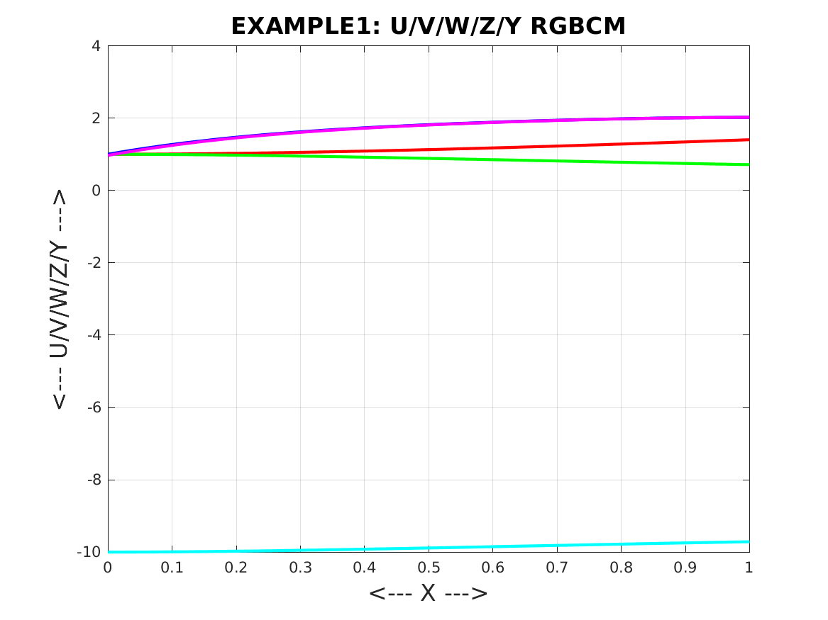
EXAMPLE 1 sets up a solution to a system of five first order ODE's. This is a sample problem for the MUSN program.
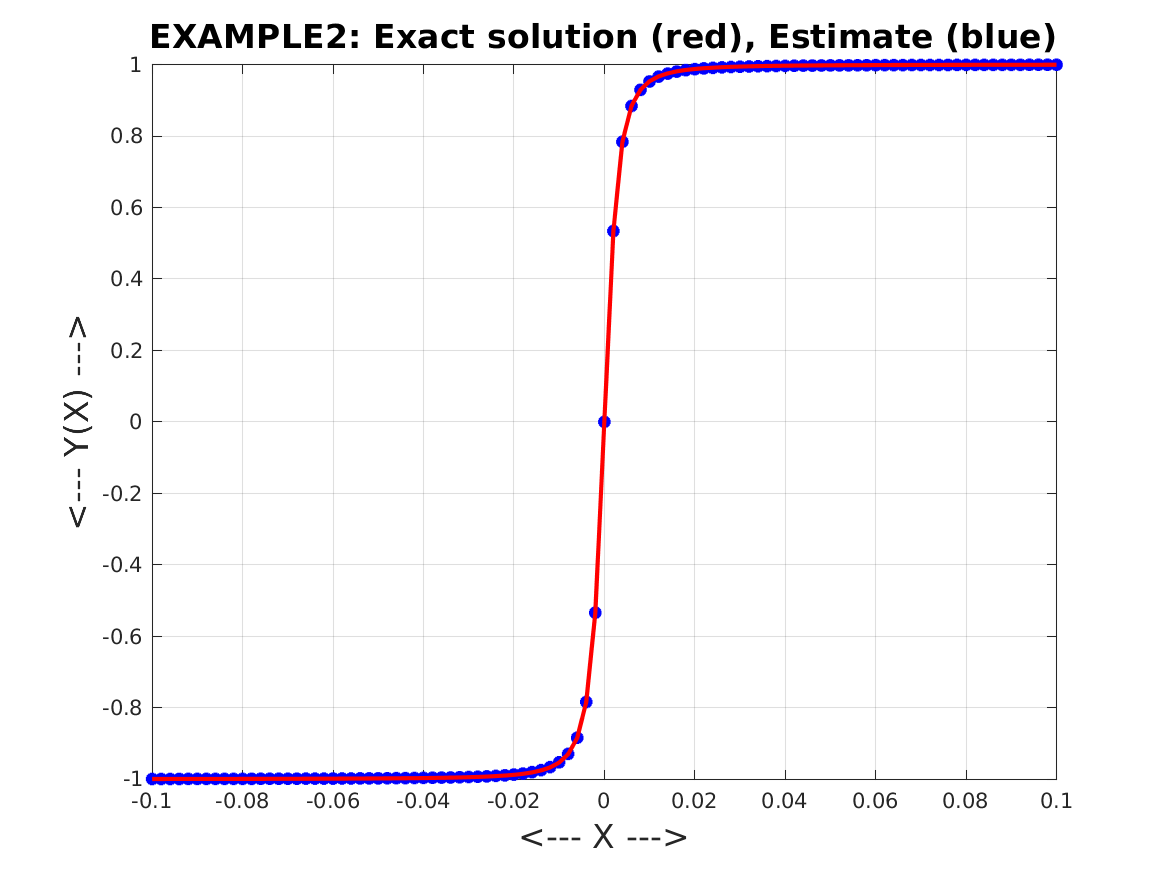
EXAMPLE 2 sets up a solution to a y''+3py/(p+x^2)^2=0, for which an analytic solution is known.
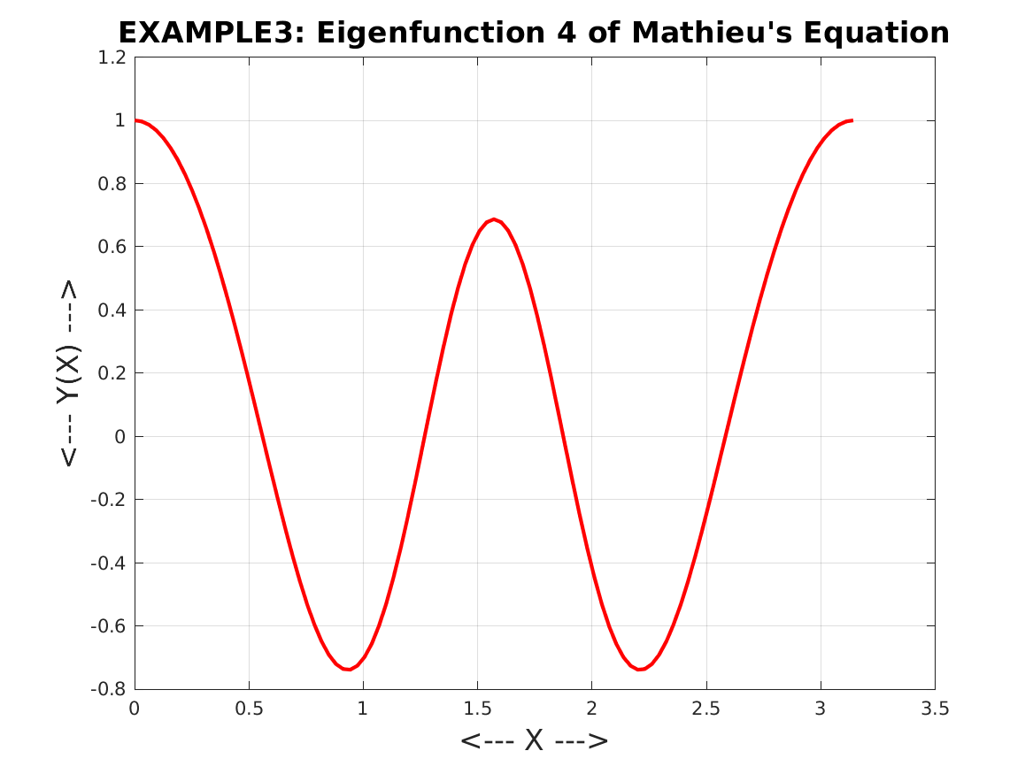
EXAMPLE 3 sets up a solution to Mathieu's equation, an eigenvalue problem y'' + (lambda-2*q*cos(2x)y)=0, y'(0) = 0, y'(pi) = 0, y(0) = 1, with q = 5, and lambda an unknown eigenvalue which we estimate to be 15. The special functional form is used to specify the initial guess for the solution.
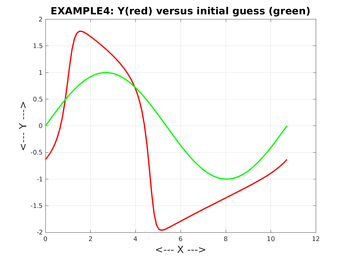
EXAMPLE 4 sets up problem modeling the propagation of nerve impulses, in which the solution is expected to be periodic, with the period unknown.
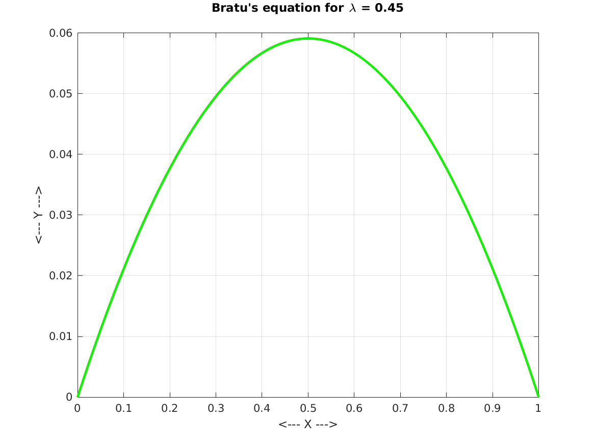
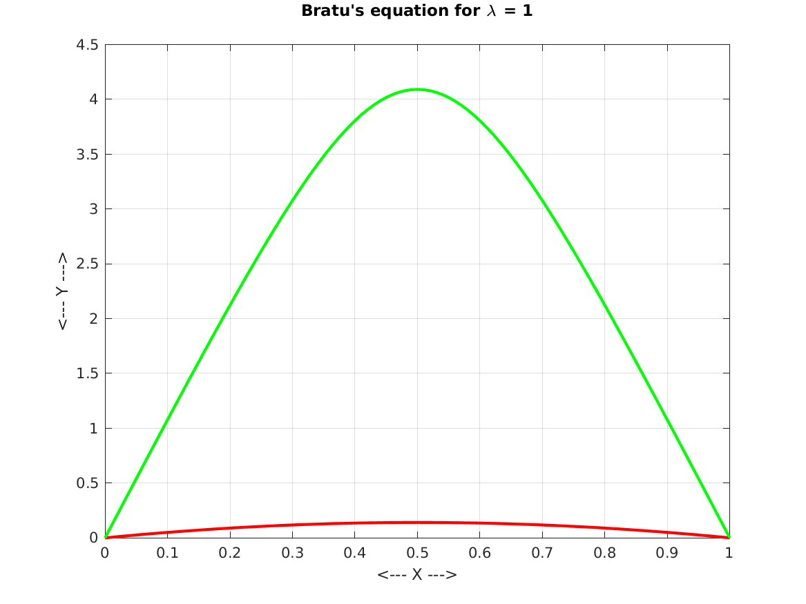
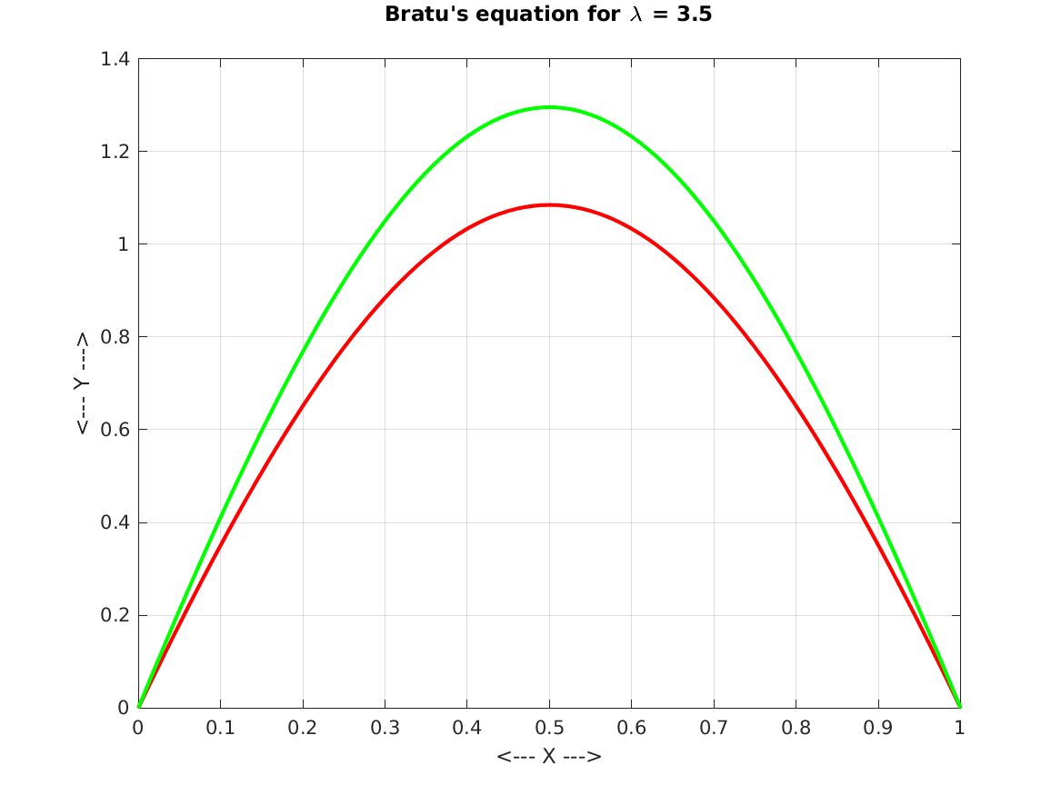
BRATU sets up the Bratu equation, which includes a parameter lambda. Depending on the value of lambda, the equation may have 2, 1 or 0 solutions.