mitchell_04

mitchell_04, a FreeFem++ code which sets up and solves Mitchell's problem #4, the Peak.

Licensing:

The computer code and data files described and made available on this web page are distributed under the MIT license

Reference:

A web site at NIST describes these and many other problems: http://math.nist.gov/amr-benchmark/index.html

1. Frederic Hecht,
   New development in FreeFem++,
   Journal of Numerical Mathematics,
   Volume 20, Number 3-4, 2012, pages 251-265.
2. William Mitchell,
   A collection of 2D elliptic problems for testing adaptive grid refinement algorithms,
   Applied Mathematics and Computation,
   Volume 220, 1 September 2013, pages 350-364.
3. Pedro Morin, Ricardo Nochetto, Kunibert Siebert,
   Data oscillation and convergence of adaptive FEM,
   SIAM Journal on Numerical Analysis,
   Volume 38, Number 2, 2000, pages 466-488.

Source code:

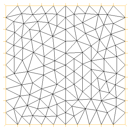
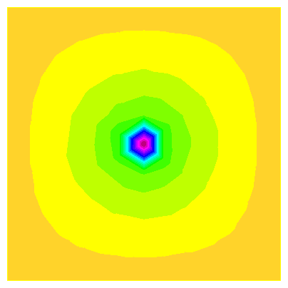
mitchell_04a defines the "peak" problem on the [0,+1]x[0,+1] square, using parameters XC = 0.5, YC = 0.5, ALPHA = 1000.

• mitchell_04a.edp, the input file.
• mitchell_04a.sh, runs FreeFem++ on the input file.
• mitchell_04a.txt, the output file.
• mitchell_04a_mesh.png, a PNG image of the mesh.
• mitchell_04a_u.png, a PNG image of a contour plot of the solution.

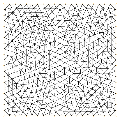
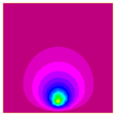
mitchell_04b defines the "peak" problem on the [0,+1]x[0,+1] square, using parameters XC = 0.51, YC = 0.117, ALPHA = 100000.

• mitchell_04b.edp, the input file.
• mitchell_04b.sh, runs FreeFem++ on the input file.
• mitchell_04b.txt, the output file.
• mitchell_04b_mesh.png, a PNG image of the mesh.
• mitchell_04b_u.png, a PNG image of a contour plot of the solution.

TEST05 defines the "battery" problem. This problem is defined on a rectangle which has been subdivided into seven subregions. Because of the complicated internal walls, it was expedient to create the mesh beforehand with BAMG.

• battery_g.msh, the BAMG geometry file file.
• battery_o.msh, the BAMG mesh file.
• battery_convert.edp, a FreeFem++ script which converts the BAMG geometry and mesh files into a FreeFem++ mesh file.
• battery.msh, the FreeFem++ mesh file.
• test05.edp, the input file.
• test05.sh, runs FreeFem++ on the input file.

TEST06A defines the "boundary layer" problem on the [-1,+1]x[-1,+1] square, using the parameter EPS = 0.1.

• test06a.edp, the input file.
• test06a.sh, runs FreeFem++ on the input file.
• test06a.txt, the output file.
• test06a_mesh.png, a PNG image of the mesh.
• test06a_u.png, a PNG image of a contour plot of the solution.

TEST06B defines the "boundary layer" problem on the [-1,+1]x[-1,+1] square, using the parameter EPS = 0.001. The only difference from TEST06A is the value of EPS, but this test fails to run at all. Even EPS=0.01 won't run.

• test06b.edp, the input file.
• test06b.sh, runs FreeFem++ on the input file.
• test06b.txt, the output file.
• test06b_mesh.png, a PNG image of the mesh.
• test06b_u.png, a PNG image of a contour plot of the solution.

TEST07 defines the "boundary line singularity" problem on the [0,+1]x[0,+1] square. There is a singularity in the right hand side function F(X,Y), at the left boundary. We use the parameter value ALPHA = 0.6.

• test07.edp, the input file.
• test07.sh, runs FreeFem++ on the input file.
• test07.txt, the output file.
• test07_mesh.png, a PNG image of the mesh.
• test07_u.png, a PNG image of a contour plot of the solution.

TEST08a defines the "oscillatory" problem on the [0,+1]x[0,+1] square, using parameter ALPHA = 1 / ( 10 * PI ).

• test08a.edp, the input file.
• test08a.sh, runs FreeFem++ on the input file.
• test08a.txt, the output file.
• test08a_mesh.png, a PNG image of the mesh.
• test08a_u.png, a PNG image of a contour plot of the solution.

TEST08b defines the "oscillatory" problem on the [0,+1]x[0,+1] square, using parameter ALPHA = 1 / ( 50 * PI ).

• test08b.edp, the input file.
• test08b.sh, runs FreeFem++ on the input file.
• test08b.txt, the output file.
• test08b_mesh.png, a PNG image of the mesh.
• test08b_u.png, a PNG image of a contour plot of the solution.

TEST09a defines the "wave front" problem on the [0,+1]x[0,+1] square with parameters ALPHA = 20, XC = -0.05, YC = -0.05, R0 = 0.7.

• test09a.edp, the input file.
• test09a.sh, runs FreeFem++ on the input file.
• test09a.txt, the output file.
• test09a_mesh.png, a PNG image of the mesh.
• test09a_u.png, a PNG image of a contour plot of the solution.

TEST09b defines the "wave front" problem on the [0,+1]x[0,+1] square with parameters ALPHA = 1000, XC = -0.05, YC = -0.05, R0 = 0.7.

• test09b.edp, the input file.
• test09b.sh, runs FreeFem++ on the input file.
• test09b.txt, the output file.
• test09b_mesh.png, a PNG image of the mesh.
• test09b_u.png, a PNG image of a contour plot of the solution.

TEST09c defines the "wave front" problem on the [0,+1]x[0,+1] square with parameters ALPHA = 1000, XC = 1.5, YC = 0.25, R0 = 0.92.

• test09c.edp, the input file.
• test09c.sh, runs FreeFem++ on the input file.
• test09c.txt, the output file.
• test09c_mesh.png, a PNG image of the mesh.
• test09c_u.png, a PNG image of a contour plot of the solution.

TEST09d defines the "wave front" problem on the [0,+1]x[0,+1] square with parameters ALPHA = 50, XC = 0.5, YC = 0.5, R0 = 0.25.

• test09d.edp, the input file.
• test09d.sh, runs FreeFem++ on the input file.
• test09d.txt, the output file.
• test09d_mesh.png, a PNG image of the mesh.
• test09d_u.png, a PNG image of a contour plot of the solution.

TEST10a defines the "interior line singularity" problem on the [-1,+1]x[-1,+1] square with parameters ALPHA = 2.5, BETA = 0.0.

• test10a.edp, the input file.
• test10a.sh, runs FreeFem++ on the input file.
• test10a.txt, the output file.
• test10a_mesh.png, a PNG image of the mesh.
• test10a_u.png, a PNG image of a contour plot of the solution.

TEST10b defines the "interior line singularity" problem on the [-1,+1]x[-1,+1] square with parameters ALPHA = 1.1, BETA = 0.0.

• test10b.edp, the input file.
• test10b.sh, runs FreeFem++ on the input file.
• test10b.txt, the output file.
• test10b_mesh.png, a PNG image of the mesh.
• test10b_u.png, a PNG image of a contour plot of the solution.

TEST10c defines the "interior line singularity" problem on the [-1,+1]x[-1,+1] square with parameters ALPHA = 1.5, BETA = 0.6.

• test10c.edp, the input file.
• test10c.sh, runs FreeFem++ on the input file.
• test10c.txt, the output file.
• test10c_mesh.png, a PNG image of the mesh.
• test10c_u.png, a PNG image of a contour plot of the solution.

TEST11 defines the "intersecting interfaces" problem on the [-1,+1]x[-1,+1] square.

• test11.edp, the input file.
• test11.sh, runs FreeFem++ on the input file.
• test11.txt, the output file.
• test11_mesh.png, a PNG image of the mesh.
• test11_u.png, a PNG image of a contour plot of the solution.

TEST12 defines the "multiple difficulties" problem, on the "upside down L" shaped region.

• test12.edp, the input file.
• test12.sh, runs FreeFem++ on the input file.