Introduction
The Navier-Stokes equations describe the motion of a fluid. The non-dimensional equations for an incompressible fluid on the domain $\Omega$ with boundary $\Gamma$, over the time interval $[0,T]$, are given by: \begin{align} &\mathbf{u}_t -\nu\Delta \mathbf{u} + \mathbf{u}\cdot\nabla\mathbf{u} + \nabla p = \mathbf{f}(\mathbf{x},t)\label{eq:ns_1}\\ &\nabla\cdot\mathbf{u} = 0\label{eq:ns_2}\\ &\mathbf{u}(\mathbf{x},t) = \mathbf{g}(\mathbf{x},t) & \text{on }\Gamma \label{eq:bc}\\ &\mathbf{u}(\mathbf{x},0) = \mathbf{u}_0(\mathbf{x}) &\text{on } \Omega \label{eq:ic} \end{align} where:- $\mathbf{u}$ is the velocity of the fluid. In 2D $\mathbf{u} = \langle u, v\rangle$
- $p$ is the fluid pressure
- $\mathbf{f}(\mathbf{x},t)$ is a known forcing function
- $\mathbf{g}(\mathbf{x},t)$ is the boundary condition
- $\mathbf{u}_0(\mathbf{x})$ is the initial condition
- $\nu$ is the kinematic viscosity of the fluid
Linearization
Since \eqref{eq:ns_1} is nonlinear, we would like to linearize it. Given an initial guess $\{\mathbf{u}^0, p^0\}$ we will use Newton's method to create a sequence of iterates $\{\mathbf{u}^1, p^1\}, \{\mathbf{u}^2, p^2\}, \cdots$ that approach the actual solution of \eqref{eq:ns_1} and \eqref{eq:ns_2}. Newton's method can be written in the abstract form: \[ H'(X,\delta X) = -H(X).\] We use the definition of the Gâteaux derivative for functions: \[ H'(X,\delta X) = \lim_{\epsilon \to 0}\frac{H(X + \epsilon\delta X) - H(X)}{\epsilon}\] in Newton's method, where:- $H(X) = \mathbf{u}_t -\nu\Delta\mathbf{u}^{(k)} + \mathbf{u}^{(k)}\cdot\nabla\mathbf{u}^{(k)} + \nabla p^{(k)} - \mathbf{f}$
- $X = \{\mathbf{u}^{(k)}, p^{(k)}\}$
- $\delta X = \{\delta\mathbf{u}, \delta p\} = \{\mathbf{u}^{(k+1)} - \mathbf{u}^{(k)}, p^{(k+1)} - p^{(k)}\}$
Weak Formulation
To obtain the Galerkin weak formulation we will take the inner product (assuming it exists) of \eqref{eq:ns_linear} with a test function $\mathbf{v} \in \mathbf{H}^1_0$ and then integrate by parts to get: \begin{equation}\label{eq:ns_weak1} (\mathbf{u}^{k+1}_t, v) + a(\mathbf{u}^{k+1},\mathbf{v}) + c(\mathbf{u}^{k+1}, \mathbf{u}^k, \mathbf{v}) + c(\mathbf{u}^k, \mathbf{u}^{k+1}, \mathbf{v}) + b(\mathbf{v}, p^{k+1}) = (\mathbf{f}, \mathbf{v}) + c(\mathbf{u}^k,\mathbf{u}^k,\mathbf{v}) \end{equation} where:- $a(\mathbf{u},\mathbf{v}) = \nu\int_\Omega \nabla\mathbf{u}:\nabla\mathbf{v} \text{d}\Omega$
- $b(\mathbf{u}, p) = -\int_\Omega p\nabla\cdot\mathbf{u} \text{d}\Omega$
- $c(\mathbf{u}, \mathbf{v}, \mathbf{w}) = \int_\Omega \mathbf{u}\cdot\nabla\mathbf{v}\cdot\mathbf{w} \text{d}\Omega$
- $(u,\mathbf{v}) = \int_\Omega \mathbf{u}\cdot\mathbf{v}\text{d}\Omega$
We can linearize these equations using \eqref{eq:ns_linear}: \begin{align*} (\mathbf{u}^{(k+1)}_t,\mathbf{v}) + a(\mathbf{u}^{(k+1)},\mathbf{v}) + c(\mathbf{u}^{(k+1)},\mathbf{u}^{(k)},\mathbf{v}) + c(\mathbf{u}^{(k)},\mathbf{u}^{(k+1)},\mathbf{v}) \\\qquad\qquad + b(\mathbf{v},p^{(k+1)}) &= (\mathbf{f},\mathbf{v}) + c(\mathbf{u}^{(k)},\mathbf{u}^{(k)},\mathbf{v}) &\text{ for all } \mathbf{v}\in \mathbf{H}^1_0(\Omega)\\ b(\mathbf{u}^{k+1},q) &= 0 &\text{ for all } q\in L^2(\Omega) \end{align*}
Time Discretization
We can discretize the time derivative $\mathbf{u}^{(k+1)}_t$ with the $\theta$ method. Let $\mathbf{u}^{n,(k)}$ be the $k$-th Newton iteration for $\mathbf{u}(\mathbf{x},\delta)$. Then for $0\leq\theta\leq 1$, the $\theta$ method is given by: \[ \left(\frac{\mathbf{u}^{n+1,(k+1)} -\mathbf{u}^{n}}{\delta},\mathbf{v}\right) + b(\mathbf{v},p^{n+1,(k+1)}) = \theta F_1(\mathbf{u}^{n+1,(k+1)},\mathbf{u}^{n+1,(k)},\mathbf{v})) + (1-\theta)F_2(\mathbf{u}^{n},\mathbf{v}),\] where: \begin{align*} F_1(\mathbf{u}^{n+1,(k+1)},\mathbf{u}^{n+1,(k)},\mathbf{v})) &= \mathbf{f}(\mathbf{x},(n+1)\delta) - a(\mathbf{u}^{n+1,(k+1)},\mathbf{v}) - c(\mathbf{u}^{n+1,(k+1)},\mathbf{u}^{n+1,(k)},\mathbf{v}) \\ \qquad\qquad &- c(\mathbf{u}^{n+1,(k)},\mathbf{u}^{n+1,(k+1)},\mathbf{v}) + c(\mathbf{u}^{n+1,(k)},\mathbf{u}^{n+1,(k)},\mathbf{v})\\ F_2(\mathbf{u}^{n},\mathbf{v}) &= \mathbf{f}(\mathbf{x},n\delta) - a(\mathbf{u}^{n},\mathbf{v}) - c(\mathbf{u}^{n},\mathbf{u}^{n},\mathbf{v}) \end{align*}This is a sequence of linear systems to solve at each timestep. The initial condition \eqref{eq:ic} provides $\mathbf{u}^{0,(0)}$, meanwhile the solution from timestep $n-1$ forms the initial guess $\mathbf{u}^{n,(0)}$ for the Newton sequence at time $n\delta$.
Note the $\theta$ method is the backwards Euler method for $\theta=1$, and the Crank-Nicolson method for $\theta=0.5$. For $\theta=0.5$ this method has accuracy $O(\delta^2)$, while for $\theta\ne 0.5$ it has accuracy $O(\delta)$.
Discrete Formulation
To form a linear system, let $\mathbf{U} = \sum\limits_{j=1}^J \alpha_j(t)\mathbf{v}_j(\mathbf{x})$ and $P = \sum\limits_{m=1}^M \beta_m(t) q_m(\mathbf{x})$ be approximations to $\mathbf{u}$ and $p$ respectively. If we assume that $\{\mathbf{v}_j\}$ $j=1,\cdots,J$ forms a basis for a finite dimensional subset of $\mathbf{H}^1$ and $\{q_m\}$, $m = 1,\cdots,M$ forms a basis for a finite dimensional subset of $L^2$, then we can write \eqref{eq:ns_weak1} and \eqref{eq:ns_weak2} as: \begin{equation}\label{eq:ns_weak3} \begin{aligned} &\left(\frac{\mathbf{U}^{n+1,(k+1)} -\mathbf{U}^{n}}{\delta},\mathbf{v}_i\right) + b(\mathbf{v}_i,P^{n+1,(k+1)}) = \theta F_1(\mathbf{U}^{n+1,(k+1)},\mathbf{U}^{n+1,(k)},\mathbf{v}_i)) + (1-\theta)F_2(\mathbf{U}^{n},\mathbf{v}_i) \qquad i = 1, \cdots, J\\ &b(\mathbf{U}^{(n+1),k+1}, q_\ell) = 0 \qquad \ell = 1,\cdots, M \end{aligned} \end{equation} This is a sequence of linear problems ($k = 1, 2, \cdots$) to solve at each time step ($n = 1, \cdots, N)$. The initial guess $U^{(n+1),0)}$ for each time step is taken as the solution from the previous time step, $U^{(n)}$. The initial conditions on the velocity determine $U^{(0),0}$. Note that no initial conditions are required for the pressure.To complete our setup we must choose the basis functions $\mathbf{v}_i$ and $q_\ell$. It turns out that a good choice that guarantees stability is the Taylor-Hood element pair. This is a mixed finite element consisting of piecewise quadratics for the velocity and piecewise linears for the pressure.
Code
A finite element solver written in C++ using the deal.ii finite element library is available here. This code supports adaptive spatial meshing and stress boundary conditions for slit flow. Meshes can be created in Gmsh.Results
Lid Driven Cavity
A common test problem in CFD is the lid driven cavity problem. In this problem we consider fluid in a box subject to a lid moving to the right with speed $U$. There are no slip boundary conditions on all the walls, so the fluid on top moves along with the lid.If we consider the unit box, with $U$ = 1, the characteristic length $L$ is 1, and the characteristic velocity is $U$. The Reynolds number $Re$ can be calculated: \[ Re = \frac{U L}{\nu} = \frac{1}{\nu}.\] Below is an animation of the magnitude of the velocity for the lid driven cavity problem at $Re=5000$ for $t\in [0,30]$ and $\mathbf{u}(\mathbf{x},0) = \mathbf{0}$:
Flow Around a Cylinder
Another common test problem is flow around a cylinder. In this problem we look at how fluid evolves as it flows around a cylinder, or in 2D, a circle. Specifically we will look at the problem 2D-3 described by Schäfer and Turek. In this setup we take the inflow and the outflow velocity to be: \[ u(y) = \frac{4U y(y-h)\sin\left(\frac{\pi t}{8}\right)}{h^2}\] where $h$ is the height of the domain, in this case $0.41$ and $U$ is the maximum speed, in this case $1.5$. All other boundaries have no slip boundary conditions. The circle is centred at $(0.2,0.2)$, with a diameter of 0.1. This is the characteristic length scale of the problem.In the paper, they calculate the lift and drag coefficients on the circle. The stress vector normal to a point on the circle is given by: \[ \mathbf{T}^{\mathbf{n}} = \langle \tau, \sigma\rangle = \pmb{\sigma}\cdot\mathbf{n},\] where $\tau$ is the component of $\mathbf{T}^{\mathbf{n}}$ tangential to the surface, $\sigma$ is the component normal to the surface and the stress tensor $\pmb{\sigma}$ is given by: \[ \pmb{\sigma} = \nu\nabla\mathbf{u} - p\mathbf{I}.\] The total drag $F_D$ and left $F_L$ on the cirlce are calculated by taking the line integral of $\mathbf{T}^{\mathbf{n}}$ over the entire circle: \[ \langle F_D, F_L\rangle = \oint_S \mathbf{T}^{\mathbf{n}} ds.\] The dimensionless lift and drag coefficients are then given by: \[ C_D = \frac{2}{U^2 L}F_D \qquad C_L = \frac{2}{U^2 L}F_L.\] For our problem $U$ is the average inflow velocity at $t=4$, which is 1.
The other quantity calculated for this problem is the pressure difference between a point directly in front of the circle, (0.15,0.2), and a point directly behind the circle, (0.25,0.2).
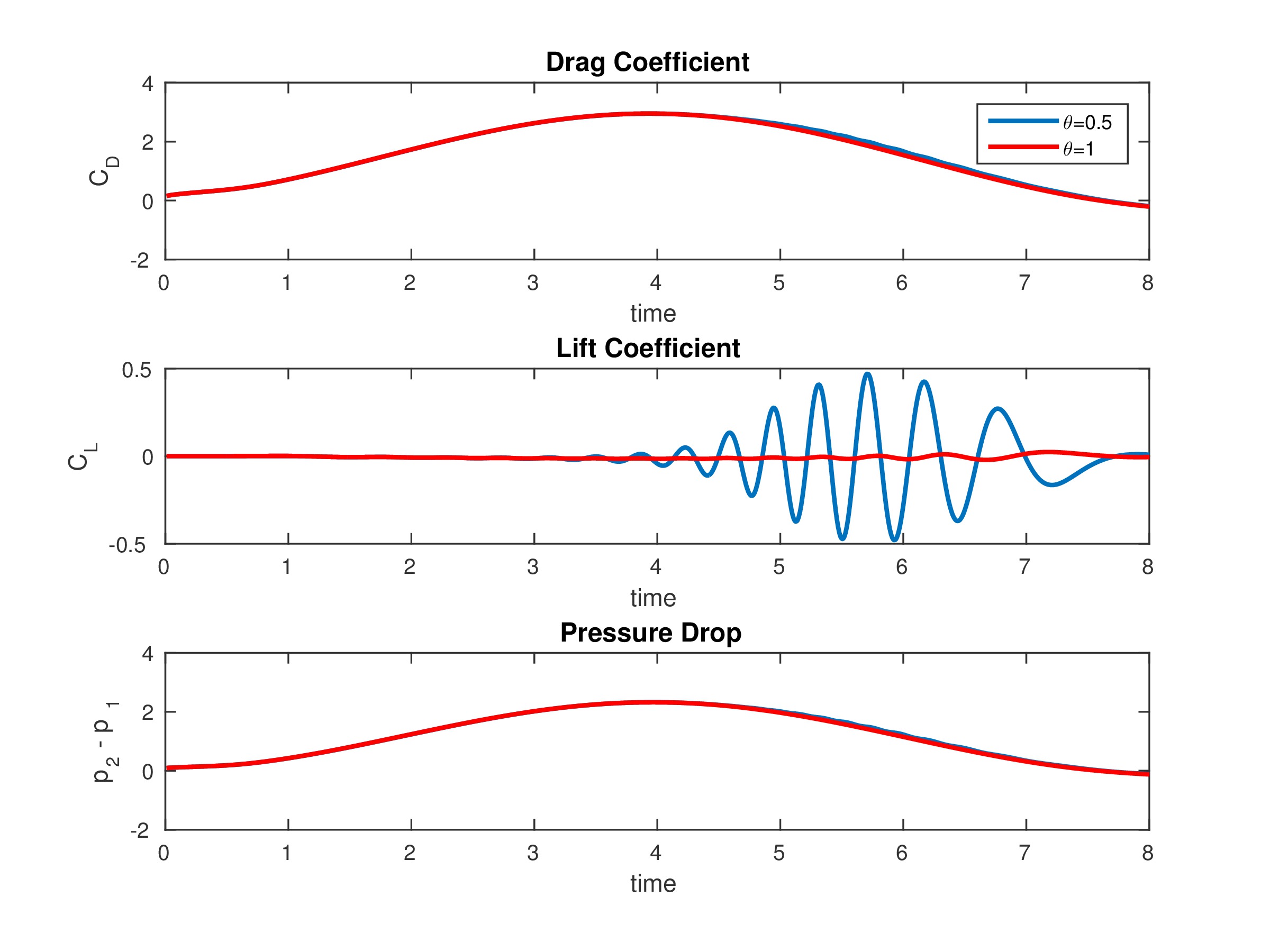
Over one half cycle from $t=0$ to $t=8$, with $\delta =0.01$, we can plot all these quantities:
 We can compare these to the results in the paper:
| max $C_D$ | max $C_L$ | $\Delta p$ | |
| $\theta = 1$ | 2.9491 | 0.0235 | -0.1245 |
| $\theta=0.5$ | 2.9495 | 0.4713 | -0.1109 |
| paper range | [2.93,2.97] | [0.47,0.49] | [-0.115, -0.105] |
For $\theta=1$, the time stepping routine is backwards Euler and is only first order in time. Consequently, it does not come close to resolving the lift. For $\theta=0.5$ the time stepping routine is the second order Crank-Nicolson method, and we find that all our values are within the range calculated in the paper.
Here is the velocity magnitude distribution for $0\leq t\leq 8$:

And here is the pressure distribution for the same time interval: