P = [3.5000 1.1100 1.1100 1.0400 1.0100;
0.5000 0.9700 0.9800 1.0500 1.0100;
0.5000 0.9900 0.9900 0.9900 1.0100;
0.5000 1.0500 1.0600 0.9900 1.0100;
0.5000 1.1600 0.9900 1.0700 1.0100;
0.5000 0.9900 0.9900 1.0600 1.0100;
0.5000 0.9200 1.0800 0.9900 1.0100;
0.5000 1.1300 1.1000 0.9900 1.0100;
0.5000 0.9300 0.9500 1.0400 1.0100;
3.5000 0.9900 0.9700 0.9800 1.0100];
[m,n] = size(P);
Pi = ones(m,1)/m;
x_unif = ones(n,1)/n;
cvx_begin
variable x_opt(n)
maximize sum(Pi.*log(P*x_opt))
sum(x_opt) == 1
x_opt >= 0
cvx_end
R_opt = sum(Pi.*log(P*x_opt));
R_unif = sum(Pi.*log(P*x_unif));
display('The long term growth rate of the log-optimal strategy is: ');
disp(R_opt);
display('The long term growth rate of the uniform strategy is: ');
disp(R_unif);
rand('state',10);
N = 10;
T = 200;
w_opt = []; w_unif = [];
for i = 1:N
events = ceil(rand(1,T)*m);
P_event = P(events,:);
w_opt = [w_opt [1; cumprod(P_event*x_opt)]];
w_unif = [w_unif [1; cumprod(P_event*x_unif)]];
end
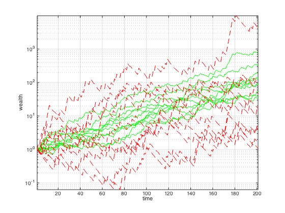
figure
semilogy(w_opt,'g')
hold on
semilogy(w_unif,'r--')
grid
axis tight
xlabel('time')
ylabel('wealth')
Successive approximation method to be employed.
   For improved efficiency, SDPT3 is solving the dual problem.
   SDPT3 will be called several times to refine the solution.
   Original size: 36 variables, 15 equality constraints
   10 exponentials add 80 variables, 50 equality constraints
-----------------------------------------------------------------
 Cones  |             Errors              |
Mov/Act | Centering  Exp cone   Poly cone | Status
--------+---------------------------------+---------
 10/ 10 | 1.166e+00  9.529e-02  0.000e+00 | Solved
 10/ 10 | 1.083e-01  9.046e-04  0.000e+00 | Solved
 10/ 10 | 2.870e-03  6.340e-07  0.000e+00 | Solved
  0/  0 | 0.000e+00  0.000e+00  0.000e+00 | Solved
-----------------------------------------------------------------
Status: Solved
Optimal value (cvx_optval): +0.0230783

The long term growth rate of the log-optimal strategy is:
    0.0231

The long term growth rate of the uniform strategy is:
    0.0114
