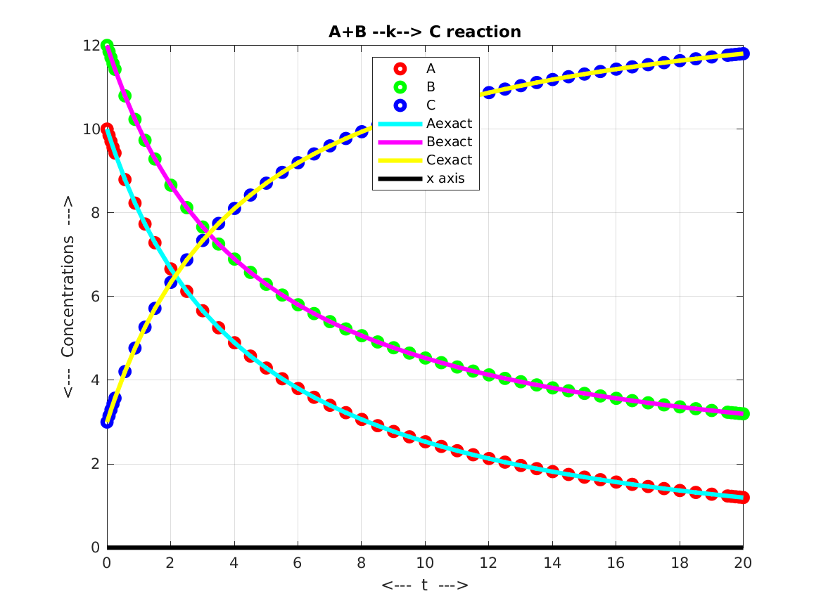
reaction_ode, a MATLAB code which defines and solves the ordinary differential equations (ODE) which model a simple chemical reaction A+B --k--> C.
The system of ODEs has the form:
        dAdt = - k A B
        dBdt = - k A B
        dCdt = + k A B
where k = 0.02 is a kind of reaction rate coefficient.
The initial conditions are taken at time T0 = 0 to be
        A = 10.0
        B = 12.0
        C =  3.0
and we are interested in approximating the solution from T0 up to TMAX = 20.
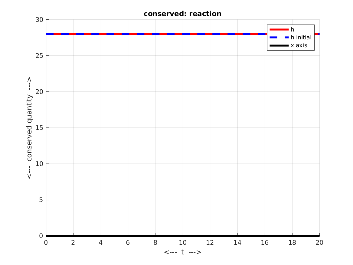
Because we can observe that dAdt + dBdt + 2 * dCdt = 0, we can define the quantity
H(t) = A(t) + B(t) + 2 C(t)
and the exact solution must satisfy H(t) = H(0), that is, H is a conserved quantity
for the exact solution.
The MATLAB ODE solver ode45() expects the variables to be stored as a single vector. So we define
y = [ a; b; c ];
The MATLAB ODE solver ode45() expects the right hand sides of the ODE to be computed by a function of the form:
      function dydt = rhs ( t, y )
        dydt = [ y1prime; y2prime; ... ]
        return
      end
so we have the function dydt = reaction_deriv ( t, y ) which does this.
When we call ode45(), the name of this right hand side function must be preceded
by an at sign (@), to indicate that it is the name of a function.
For convenience, we store the value of k and the initial condition information in the function [ k, t0, y0 ] = reaction_parameters ( ). Here, of course, y0 is a vector containing the the initial condition values a0, b0, c0 at time t0. To solve a new problem, you just need to change the values in this function.
The exact solution of this problem is known for any values of t0, y0, and is available from the function ye = reaction_exact ( t ), where t may be a single time, or a vector of times. It is useful to compare the exact solution to the computed solution.
The conserved quantity can be evaluated at y, where y is a single solution value, or a sequence of solution values at various times t, by calling h = reaction_conserved ( y ).
To have ode45() solve the problem, use a MATLAB statement like
[ t, y ] = ode45 ( tspan, deriv );
where
To plot the solution components returned by ode45(), try
plot ( t, y )
This is enough to get started, but you can do much more to make the plot prettier.
To plot the conserved quantity:
        h = reaction_conserved ( y );
        plot ( t, h )
The function reaction_ode_test() sets up the problem, solves it with ode45(), and makes plots. It includes documentation, print statements, and extra plot commands which might the output nicer. You don't need to understand all of these extra things right now, but you should be able to guess how they work.
Tests:
Plots: