ball_and_stick_display_test

ball_and_stick_display_test, a MATLAB code which demonstrates the creation of a 3D ball and stick image;

Licensing:

The information on this web page is distributed under the MIT license.

Related Data and Programs:

ball_and_stick_display, a MATLAB code which demonstrates the creation of a 3D ball and stick image;

Source Code:

• ball_and_stick_display_test.m, calls all the tests.
• ball_and_stick_display_test.sh, runs all the tests.
• ball_and_stick_display_test.txt, the output file.

BALL_AND_STICK_DISPLAY displays a ball and stick plot.

• ball_and_stick_display.png, a PNG snapshot of the 3D plot.

FIRST_ORDER_DISPLAY displays a sequence of 8 images illustrating a first order method for dealing with hyperbolic equations.

• first_order_0.png, a blank plotting field.
• first_order_1.png, a node where we have the solution.
• first_order_2.png, the region associated with the node.
• first_order_3.png, the neighboring nodes.
• first_order_4.png, fluxes are differences across the neighbors.
• first_order_5.png, a full time step is now taken.
• first_order_6.png, we have an estimate for the solution in this region.
• first_order_7.png, all the nodes can be advanced in this way.

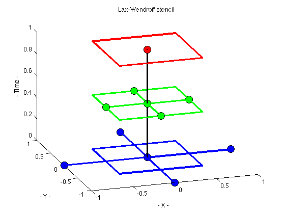
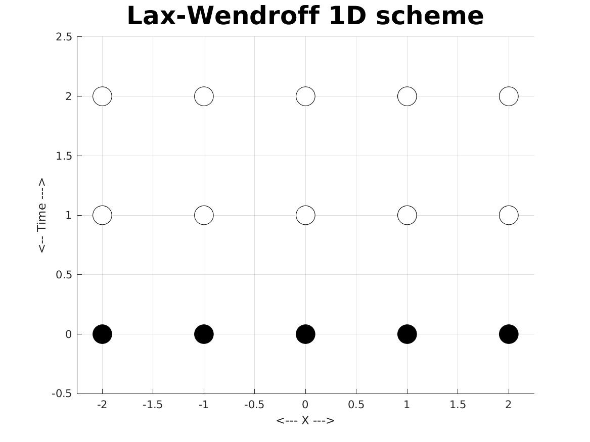
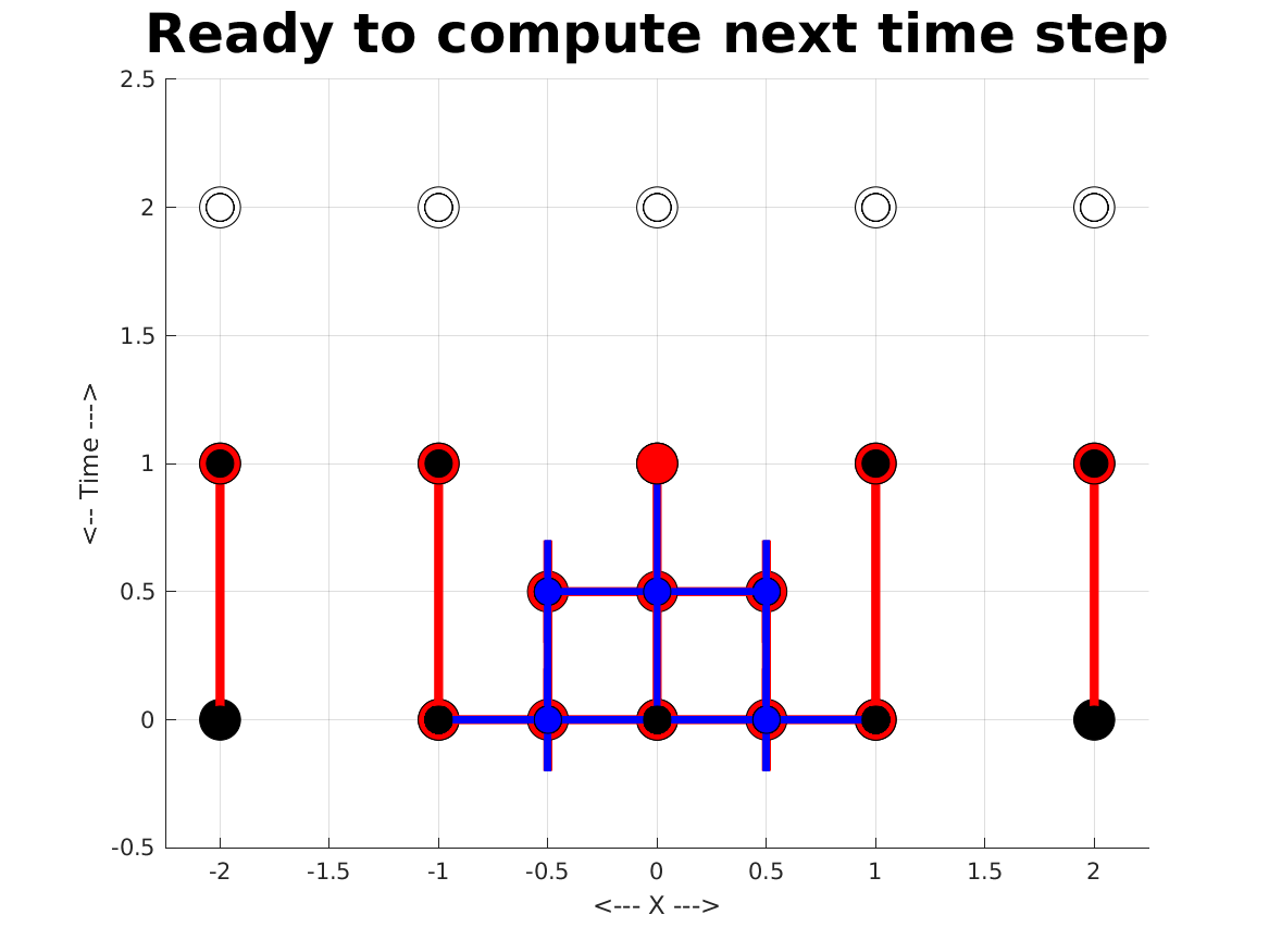
LAX_WENDROFF_1D_DISPLAY displays a sequence of images illustrating the Lax-Wendroff method in 1D.

• lw1d00.png, a blank plotting field.
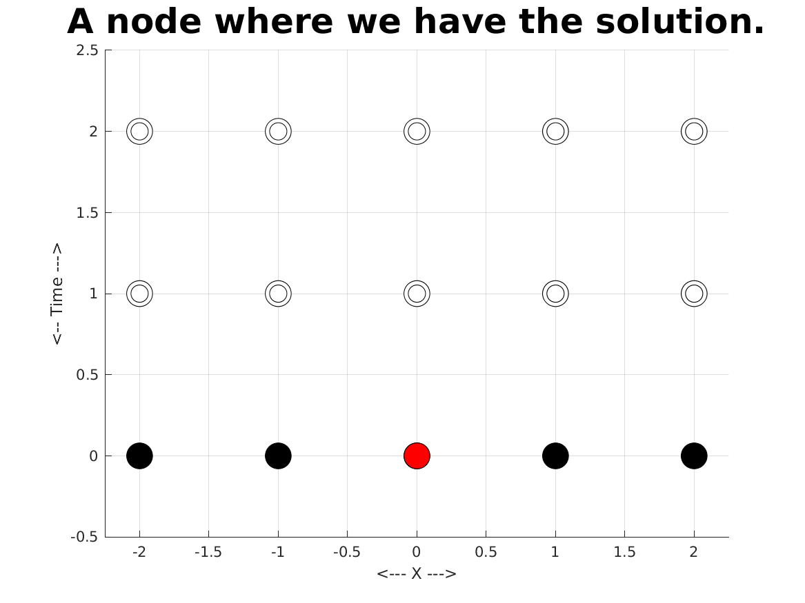
• lw1d01.png, a node where we have the solution.
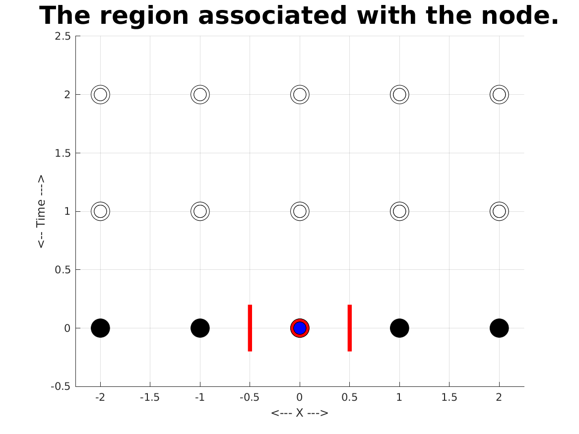
• lw1d02.png, the region associated with the node.
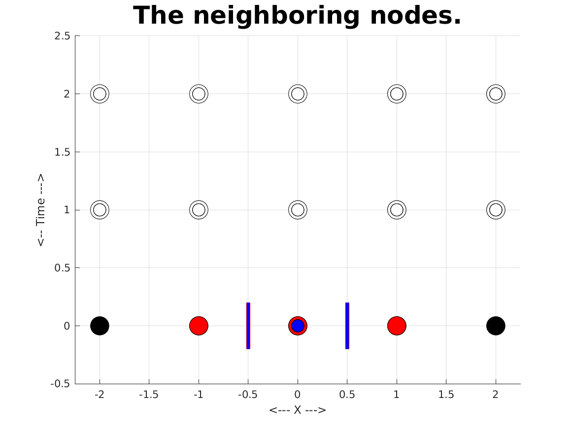
• lw1d03.png, the neighboring nodes.
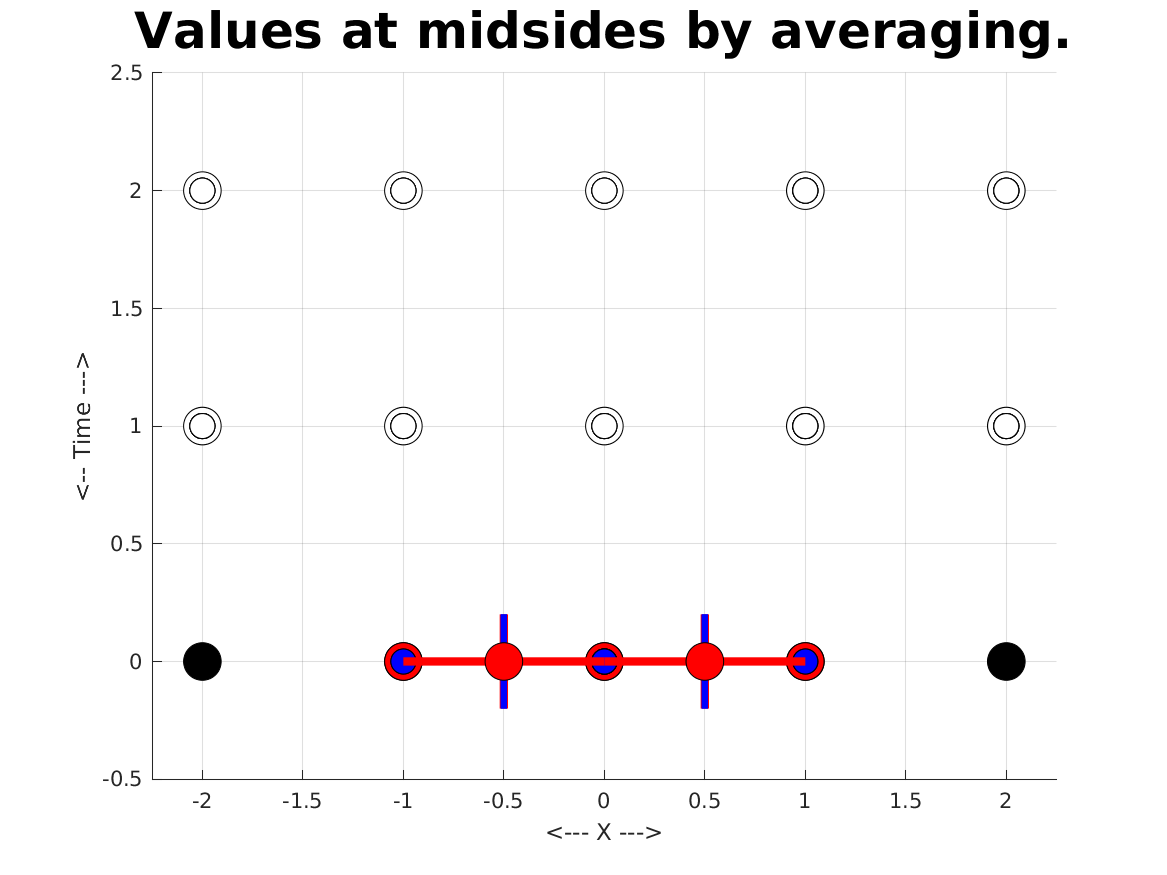
• lw1d04.png, values at midsides by averaging.
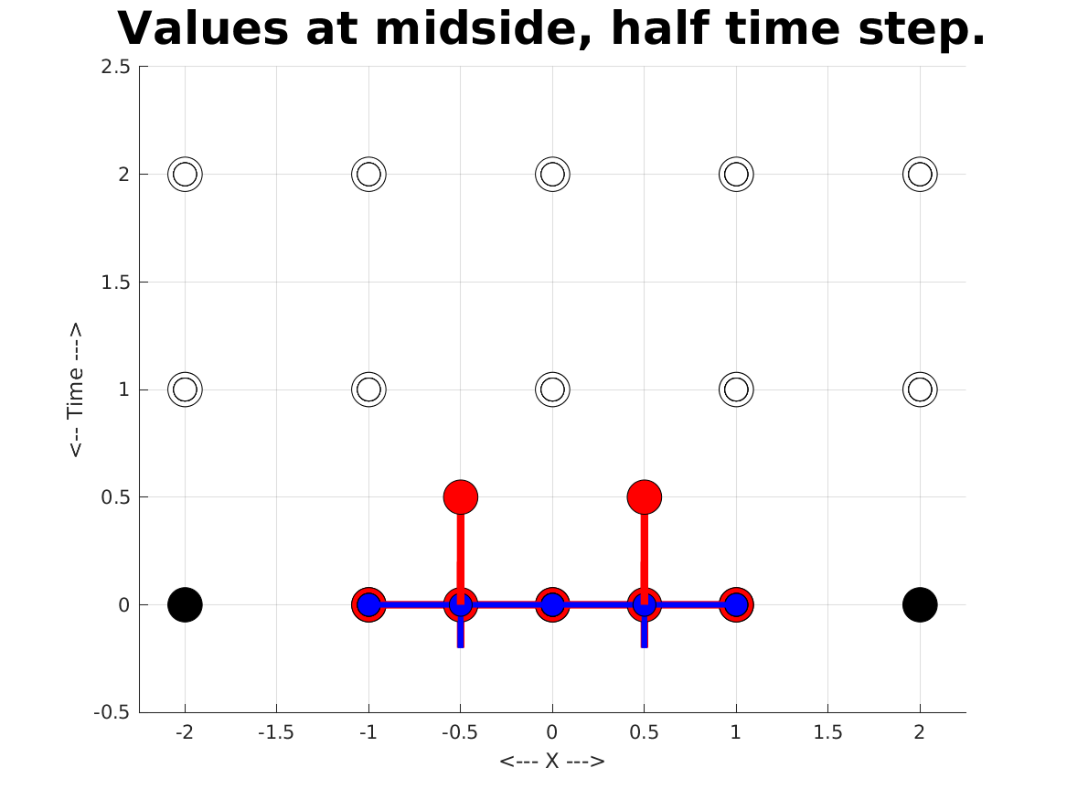
• lw1d05.png, values at midside nodes, half time step.
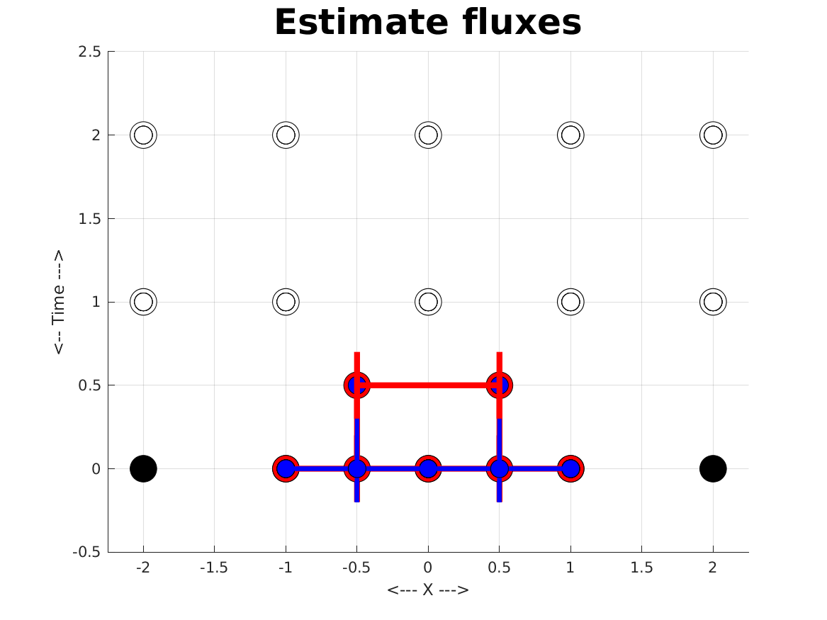
• lw1d06.png, estimate fluxes.
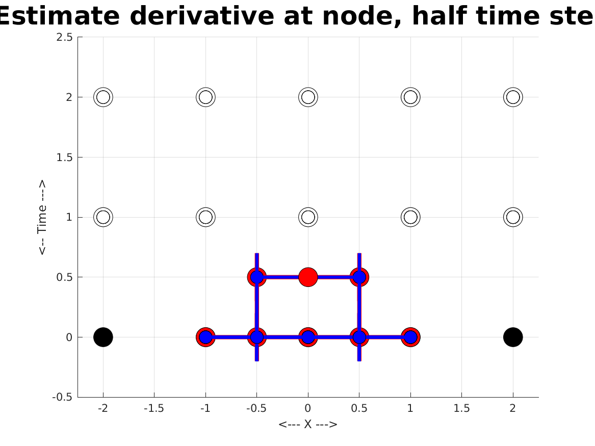
• lw1d07.png, estimate derivative at node, half time step.
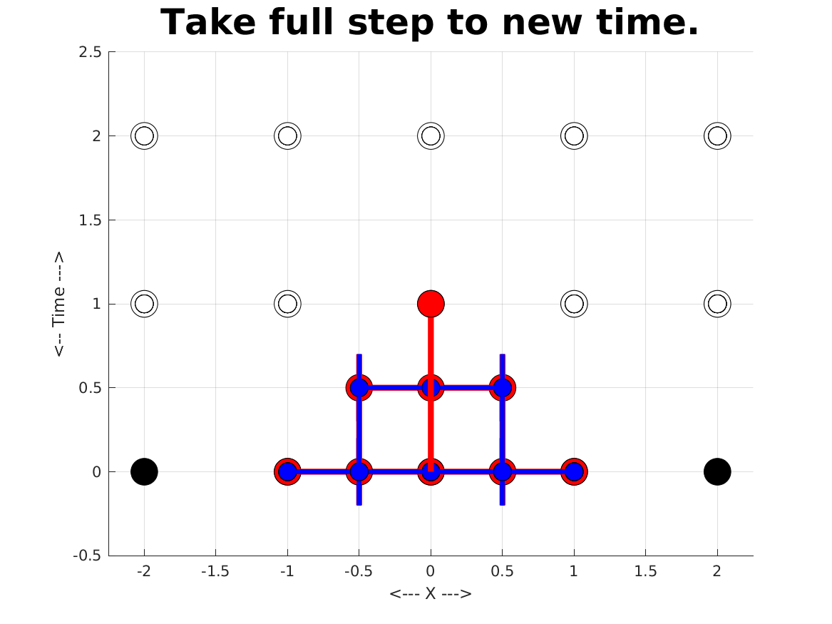
• lw1d08.png, take full step to new time.
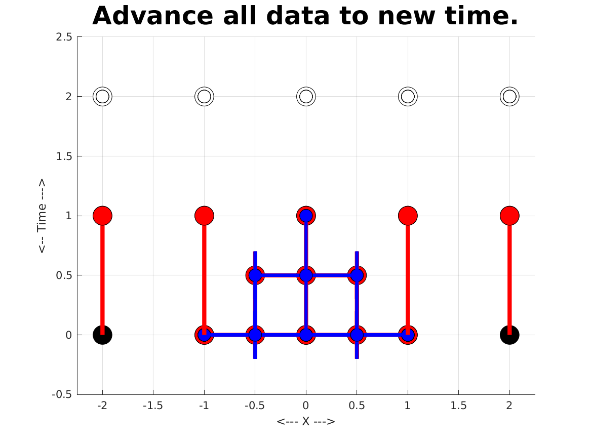
• lw1d09.png, update all data.
• lw1d10.png, ready for next time step.

LAX_WENDROFF_2D_DISPLAY displays a sequence of images illustrating the Lax-Wendroff method in 2D.

• lw2d0.png, a blank plotting field.
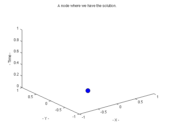
• lw2d1.png, a node where we have the solution.
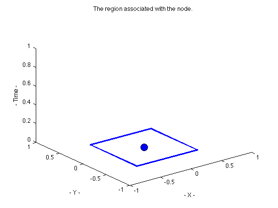
• lw2d2.png, the region associated with the node.
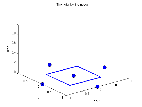
• lw2d3.png, the neighboring nodes.
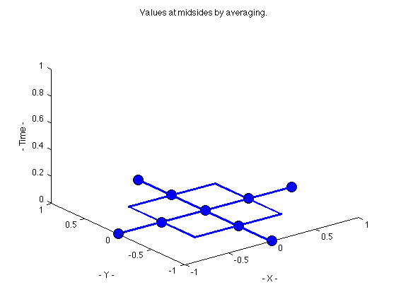
• lw2d4.png, values at midsides by averaging.
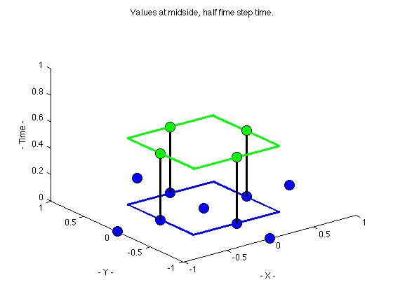
• lw2d5.png, values at midside nodes, half time step.
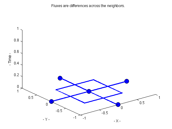
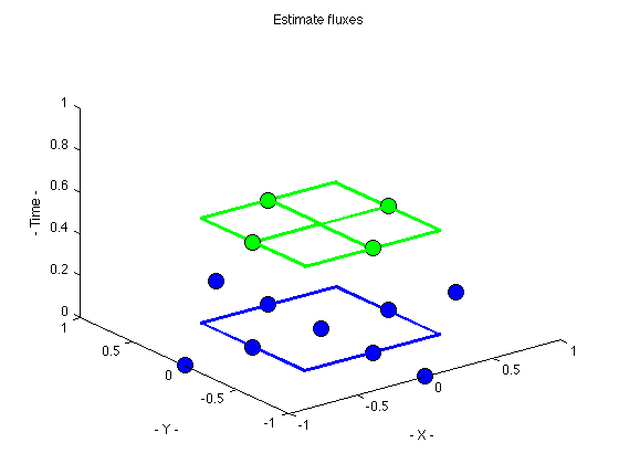
• lw2d6.png, estimate fluxes.
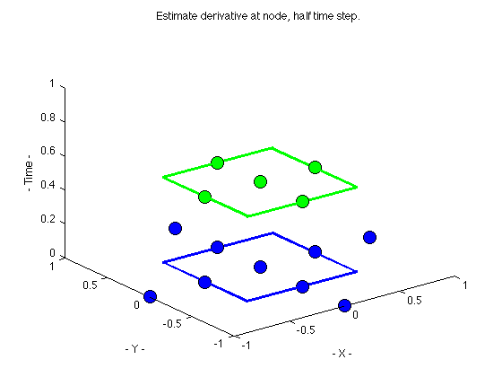
• lw2d7.png, estimate derivative at node, half time step.
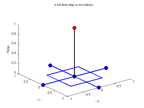
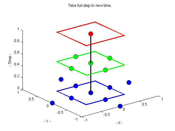
• lw2d8.png, take full step to new time.
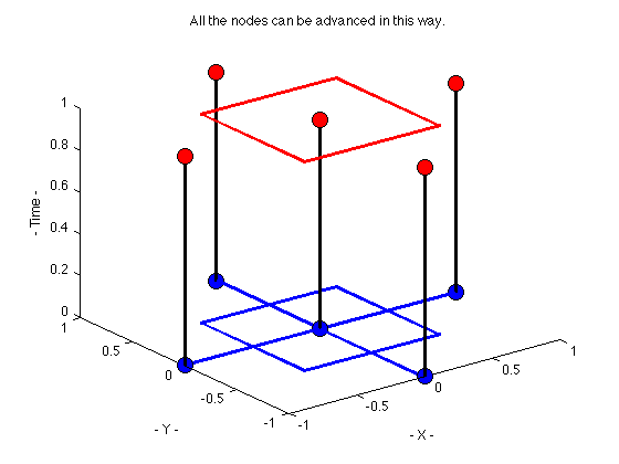
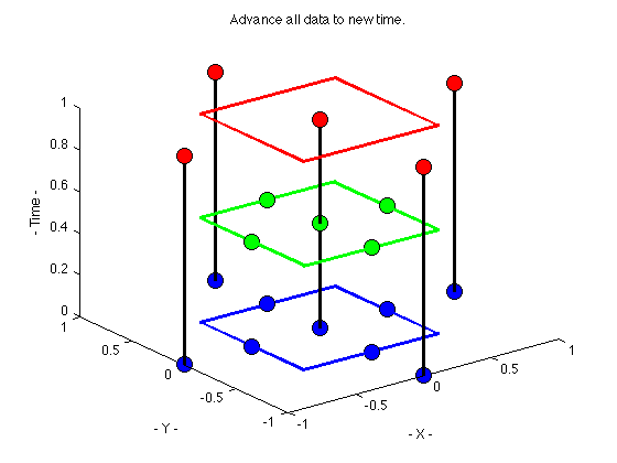
• lw2d9.png, update all data.